DVC Configuration Steps
Each panel contains a different step in the DVC configuration process. When moving between each panel, the Help section is updated. Additional help can be viewed by hovering the mouse over some of the buttons and labels on the interface.
Initial Registration
The first step of the DVC analysis is to line up the reference and correlate images. The rigid body translation between the images will be input to the DVC analysis code. Go to the Initial Registration tab to get started with this.
The Point 0 Location
First, the button Select point 0 needs to be clicked. Then, point 0 is selected by pressing “shift” and left clicking on a point in the image. Next, the size of the registration box can be edited. The slice where point 0 lies can always be visualised by clicking on the button Center on Point 0. In particular, this becomes useful after other slices of the 3D image have been visualised.
Point 0 will be used as the global starting point in the DVC analysis, as well as the reference point for the translation. Point 0 is used in the “Point Cloud” tab, where a point cloud is loaded or generated from the mask selected in the “Mask” tab. If point 0 does not lie within the mask, it will be added as the first point in the cloud.
Registering the Images
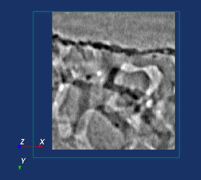
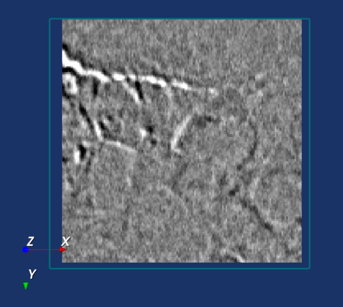
After selecting point 0 and the registration box size, the registration process is initialised by clicking on Start Registration. This runs an automatic registration procedure and the results are displayed in the widgets Translate X, Translate Y, and Translate Z, as well as in the label widget Automatic registration […]. The viewer shows an image representing the difference between the reference volume and the correlate volume. This is shown in a square with side equal to the chosen “registration box size”. The image can be spanned in 3D and it is initially centred on the slice embedding point 0. This view can be retrieved by clicking on the button Centre on Point 0. The difference image is calculated from the full-resolution volumes, not their down-sampled versions. If two volumes were identical, their difference volume would result in pixels of value 0 and the viewer would show a black square. Two images are registered optimally when their difference volume is as uniform as possible, and shown with large numbers of grey pixels in the viewer. The registration procedure can be manually adjusted by clicking on the difference image and moving the two volumes with respect to each other by using the keys: “j”, “n”, “b”, and “m”. The image orientation cab be changed using the “x”, “y” and “z” keys, and scroll through the image slices.
An example of an optimal registration is shown below, where the difference image is largely grey.
Click on the button Reset to set the translation to [0, 0, 0]. Click on the button Set to Automatic Registration to reset the translation the value of the automatic registration. Click on the button Confirm Registration when satisfied with the registration and store the translation value for the DVC analysis in the next tabs. Click on the button Cancel to terminate the registration procedure and retrieve the previous translation value. Click on the button Restart registration to restart the regitration process again.
Move to the Mask tab only when the registration has been confirmed at least once.
Mask Creation
The point cloud will be created inside a mask defined by the user. A mask is a binary image where ones represent where the points will lie. iDVC allows you to create or import a mask via file. Once satisfied with the mask, move on to the Point Cloud panel.
Creating a mask
A mask is created by tracing the cross section of the mask and extending it above and below the current slice by Slices Above and Slices Below values. More complex masks can be created by extending the mask by multiple tracing.
The user can trace in 2 modalities: free hand and or by inserting multiple segments separated by point handles.
Click on the Start Tracing button to draw a mask and enable tracing on the viewer.
Freehand tracing:
Draw a free hand line: left button click over the image, hold and drag.
Erase the line: left button click and release.
Multisegment tracing:
Start a snap drawn line: middle button click. Terminate the line by clicking the middle button while depressing the ctrl key.
Form a closed loop with the line: trace a continuous or snap drawn line and place the last cursor position close to the first handle.
Point handle dragging: right button click and hold on any handle that is part of a snap drawn line. The path can be closed by overlappingg the first and last points.
Erase any point handle: ctrl key + right button down on the handle.
Split a segment at the cursor position: shift key + right button down on any snap drawn line segment.
The 2D mask drawn in the viewer is used across multiple slices in 3D, above and below the current slice; the volume can be adjusted by editing the Slices Above and Slices Below values. Click on Create mask when the tracing is finalised.
Note: the Slices Above and Slices Below are in the coordinate system of the downsampled image (if the images have been downsampled).
Extending a mask
Tick the Extend Mask checkbox if the mask needs to cover more than one area, or the area of the mask needs to be enlarged. Then, draw another region and press the button Extend Mask.
If Extend Mask is not checked the mask will be reset when tracing.
Saving a mask
The most recent mask that has been created will automatically be applied. If it is intended to draw more than one mask click on the Save Mask button. Else, the older mask will be discarded if a new mask is created without saving the previous one.
The names of all of the saved masks will appear in a dropdown list. Each mask can be selected and reloaded by clicking on Load Saved Mask.
Note: the mask is created in the coordinate system of the down-sampled image. If the down-sampling level is changed, you may not be able to reload a mask you have previously generated.
Loading a mask from file
As an alternative to creating a mask, this may be loaded from a file by clicking Load Mask from File. The file format should be an uncompressed metaimage file, with extension ‘.mha’.
Point Cloud
Creating a point cloud
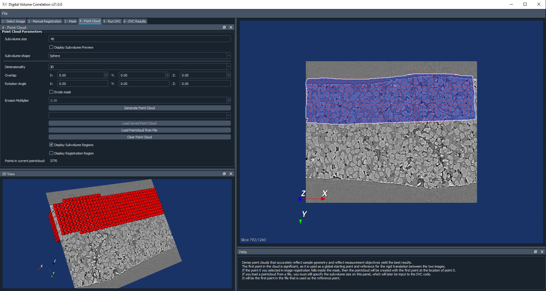
First of all, set a size for the subvolumes in the point cloud. This is the diameter of a spherical subvolume region, or the side length of a cubic one.
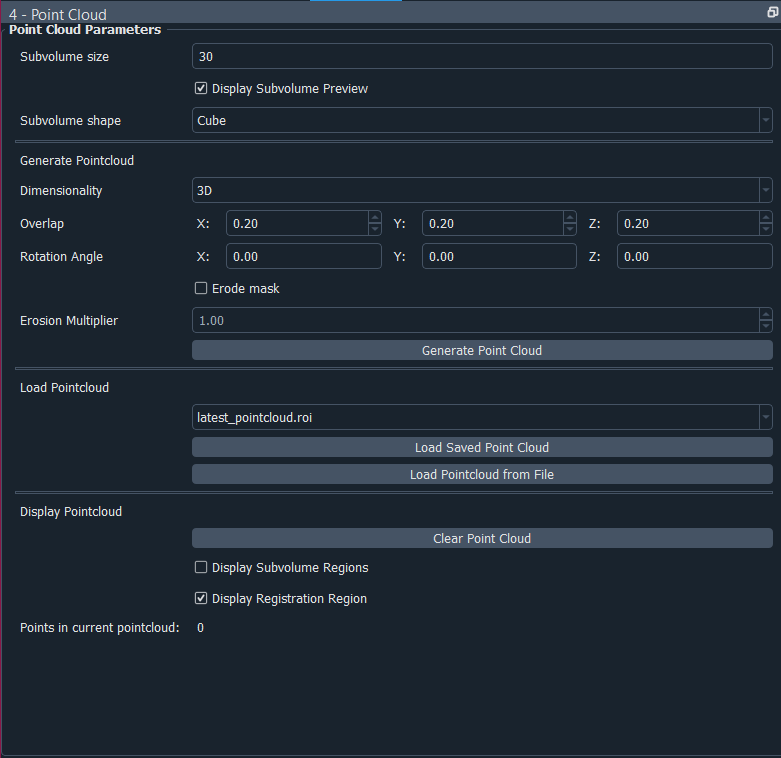
If you have ticked the option to display the subvolume preview, then a preview of the size of each subvolume will be shown in the viewer, centred on the location of the reference point 0.
If you select a 2D point cloud, then the point cloud will only be created on the currently displayed slice of the image. A 3D point cloud will be created across the entire extent of the mask.
The Overlap is the percentage overlap of the subvolume regions. You can also set a Rotation Angle of the subvolumes in degrees, relative to any of the three axes.
Parts of some of the subvolumes may lie outside of the mask, although all of the points will lie within the mask. You may choose to erode the mask by ticking Erode mask. Eroding the mask will help ensure the entirety of all of the subvolume regions lies within the mask. Be aware that this is quite a time consuming process. You may also adjust the Erosion multiplier, which will change how heavily this erosion process takes place – you may decrease the multiplier if it does not matter if some subvolumes are partially outside of the mask.
The Display Subvolume Regions option allows to turn on/off viewing the subvolumes, but the points themselves will still be displayed. The Display Registration Region toggles on/off the view of the registration box centred on point 0.
Saving and Loading a point cloud
The most recent point cloud you have created will automatically be saved, but if you would like to create a new point cloud, you will be prompted to then save the previous one, otherwise it will be discarded. The names of all of the point clouds you have saved to the current session will appear in a dropdown list. You can select one from here and reload it.
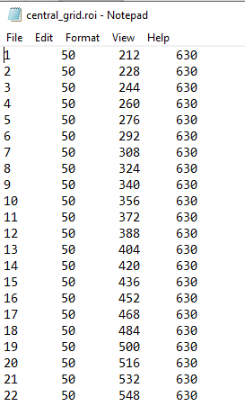
Alternatively, you may load a point cloud from a file you have saved. Allowed file formats are txt, csv, xlxs, inp. This could be a tab-delimited text file with the point number in the first column, followed by the x, y and z coordinates of each point.
An example is shown below. The first point in the file will be used as the starting point for the DVC analysis. Note that you may use non-integer coordinates.
Note that the point cloud is in the coordinate system of the original image, and is not affected by the down-sampling, it is displayed at the true location of the points. Once you are happy with your point cloud, you can move on to the Run DVC panel.
To delete a PointCloud you should press the Clear Point Cloud button.
Running the DVC Analysis
First, set a name for your run. This is how the run will be saved, and you will need to refer to this name later when you would like to view the results. The settings you can change for your run are as follows:
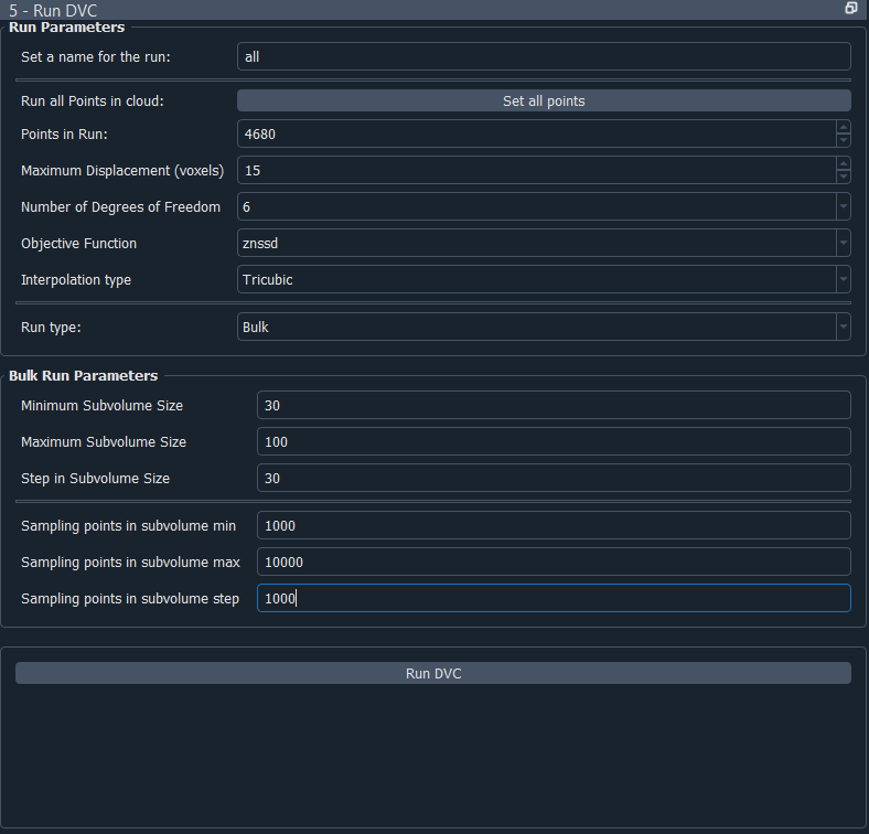
Run all Points in cloud - clicking this button resets the Points in run to all the points in the point cloud. Points in run - the number of points you would like to perform the run on. This will automatically start off being set to the total number of points in the cloud you have created, but you may wish to run with less points to begin with, as a test for instance. If you choose less points than the total number in the cloud, and your reference point 0 lies within your point cloud, the points will be selected starting with point 0 and working outwards from there.
Maximum displacement - defines the maximum displacement expected within the reference image volume. This is a very important parameter used for search process control and memory allocation. Set to a reasonable value just greater than the actual sample maximum displacement. Be cautious: large displacements make the search process slower and less reliable. It is best to reduce large rigid body displacements through image volume manipulation. Future code development will introduce methods for better management of large displacements.
Suitable values: 1 -> smallest dimension of the image volumes
Number of degrees of freedom - defines the degree-of-freedom set for the final stage of the search. The actual search process introduces degrees-of-freedom in stages up to this value. Translation only suffices for a quick, preliminary investigation. Adding rotation will significantly improve displacement accuracy in most cases. Reserve strain degrees-of-freedom for cases when the highest precision is required.
3= translation only6= translation plus rotation12= translation, rotation and strain
Objective function - defines the objective function template matching form. See B. Pan, Equivalence of Digital Image Correlation Criteria for Pattern Matching, 2010. Functions become increasingly expensive and more robust as you progress from sad to znssd. Minimizing squared-difference and maximizing cross-correlation are functionally equivalent.
sad= sum of absolute differencesssd= sum of squared differenceszssd= intensity offset insensitive sum of squared differences (value not normalized)nssd= intensity range insensitive sum of squared differences (0.0 = perfect match, 1.0 = max value)znssd= intensity offset and range insensitive sum of squared differences (0.0 = perfect match, 1.0 = max value)
Notes on objective function values:
The normalized quantities nssd and znssd are preferred, as quality of match can be assessed.
The natural range of nssd is [0.0 to 2.0], and of znssd is [0.0 to 4.0].
Both are scaled for output into the [0.0 to 1.0] range for ease of comparison.
Interpolation type - Defines the interpolation method used during template matching. Options: nearest, trilinear, tricubic.
Trilinearis significantly faster, but with known template matching artefacts.Trilinearis most useful for tuning other search parameters during preliminary runs.Tricubicis computationally expensive, but is the choice if strain is of interest.
Sampling Points in subvolume - Defines the number of points within each subvolume (max is 50000). In this code, subvolume point locations are NOT voxel-centred and the number is INDEPENDENT of subvolume size. Interpolation within the reference image volume is used to establish templates with arbitrary point locations.
For cubes a uniform grid of sampling points is generated.
For spheres, the sampling points are randomly distributed within the subvolume.
This parameter has a strong effect on computation time, so be careful. You can then either run a Single run, or a Bulk run:
A single run will run with the current point cloud you have generated, you only need to select the number of sampling points in the subvolume region.
If you select to run in bulk, this will use the loaded or generated point cloud and run dvc analysis changing the parameters subvolume size and sampling points in subvolume. You can set the minimum and maximum subvolume size you would like, and the size of the step between these values, and similar for the sampling points. In the example above, this would perform runs on point clouds with subvolume sizes 30, 60 and 90, and number of sampling points 1000, 2000, 3000, 4000, 5000, 6000, 7000, 9000 and 10000, so 30 runs in total.
For every run, any point clouds and input files to the DVC analysis code that are generated are saved in the session files, which you are able to access if you export your session (see Exporting Sessions).
Run Progress
Whilst the DVC analysis is running, you will see updates on its progress, as below:
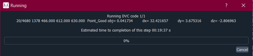
The 1/1 on the first line indicates that it is on run 1 out of a total of 1 run, and then on the next line it shows it is on point 20 out of a total of 4630 for this run. Following this we have:
[x,y,z] location of the point.
The search status:
Point_Good = successful search convergence within the max displacement.
Range_Fail = max displacement exceeded; consider increasing the disp_max parameter.
Convg_Fail = maximum iterations exceeded; consider increasing subvol_size &/or npts.
The magnitude of the objective function value at the end of the search is listed as obj=
For
obj_function = sad, ssd, and zssdthe value is relative, depending on subvolume size and pixel values.For
obj_function = nssd and znssdthe value is scaled between 0 and 2, with zero a perfect match.The point [x,y,z] displacement is listed next for successful searches.