Introduction#
The goal of the Core Imaging Library is to allow the user to simply create iterative reconstruction methods which go beyond the standard filter back projection technique and which better suit the data characteristics. The framework comprises:
cil.frameworkmodule gives the building blocks used to describe and handle the datacil.iomodule which provides a number of loaders for real CT machines, e.g. Nikon. It also provides reader and writer to save to NeXuS file format.cil.optimisationmodule allows the user to create iterative methods to reconstruct acquisition data applying different types of regularisation, which better suit the data characteristics.cil.pluginsmodule which allows CIL to use selected functionality from ASTRA, TIGRE, TomoPhantom and the Regularisation Toolkitcil.processorsmodule contains tools for data manipulation and common CT pre-processing stepscil.reconmodule contains an optimised FDK/FBP reconstructors, making using the both CIL accelerated libraries and the Tigre/ASTRA back-projectorscil.utilitiesmodule contains a selection of display tools for 2D and 3D data, as well as real and simulated test datasets
CT Geometry#
Please refer to this notebook on the CIL-Demos repository for full description.
In conventional CT systems, an object is placed between a source emitting X-rays and a detector array measuring the X-ray transmission images of the incident X-rays. Typically, either the object is placed on a rotating sample stage and rotates with respect to the source-detector assembly, or the source-detector gantry rotates with respect to the stationary object. This arrangement results in so-called circular scanning trajectory. Depending on source and detector types, there are three conventional data acquisition geometries:
parallel geometry (2D or 3D),
fan-beam geometry, and
cone-beam geometry.
Parallel geometry#
Parallel beams of X-rays are emitted onto 1D (single pixel row) or 2D detector array. This geometry is common for synchrotron sources. 2D parallel geometry is illustrated below.
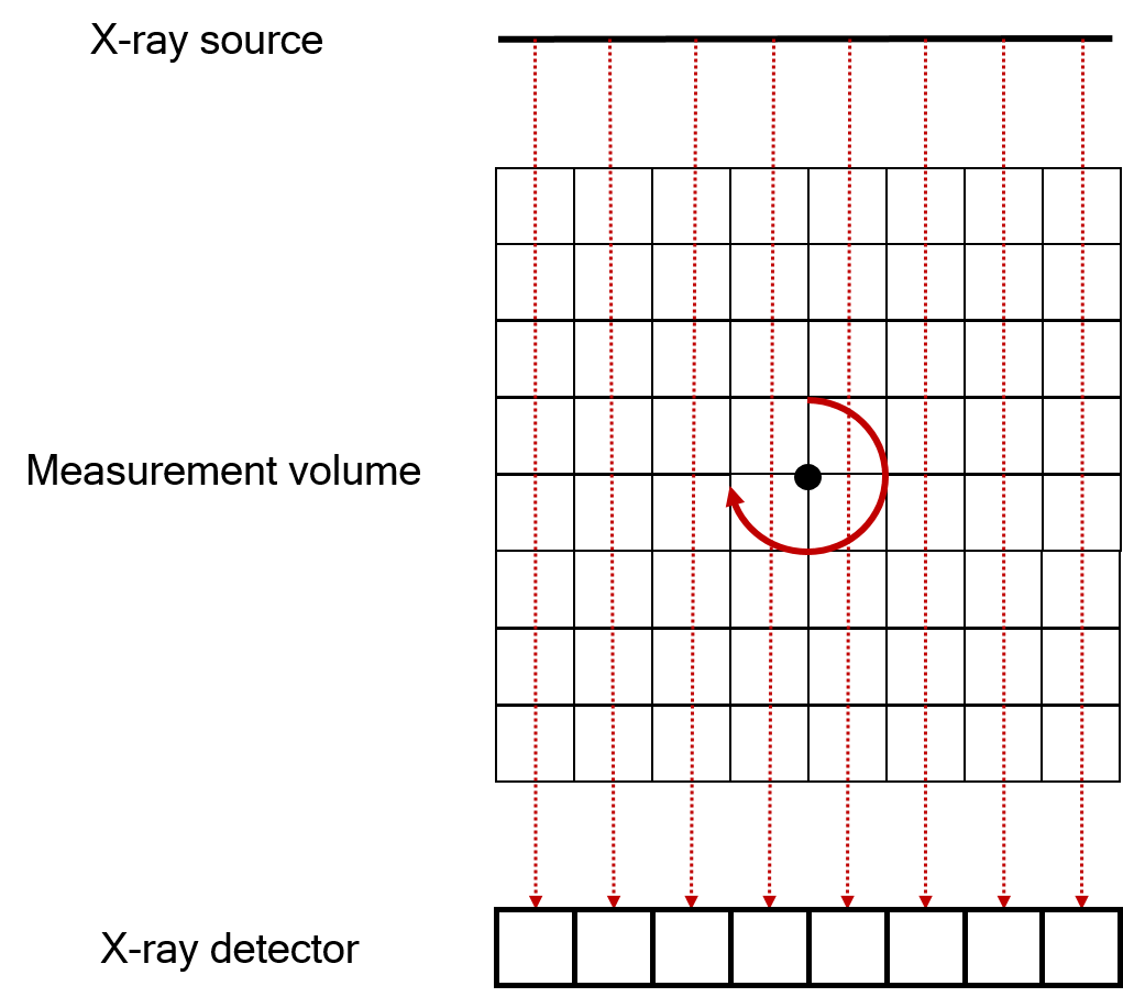
2D Parallel geometry#
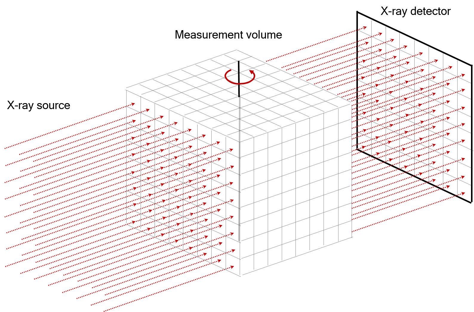
3D Parallel geometry#
Fan-beam geometry#
- A single point-like X-ray source emits a cone beam onto 1D detector pixel row. Cone-beam is typically
collimated to imaging field of view. Collimation allows greatly reduce amount of scatter radiation reaching the detector. Fan-beam geometry is used when scattering has significant influence on image quality or single-slice reconstruction is sufficient.
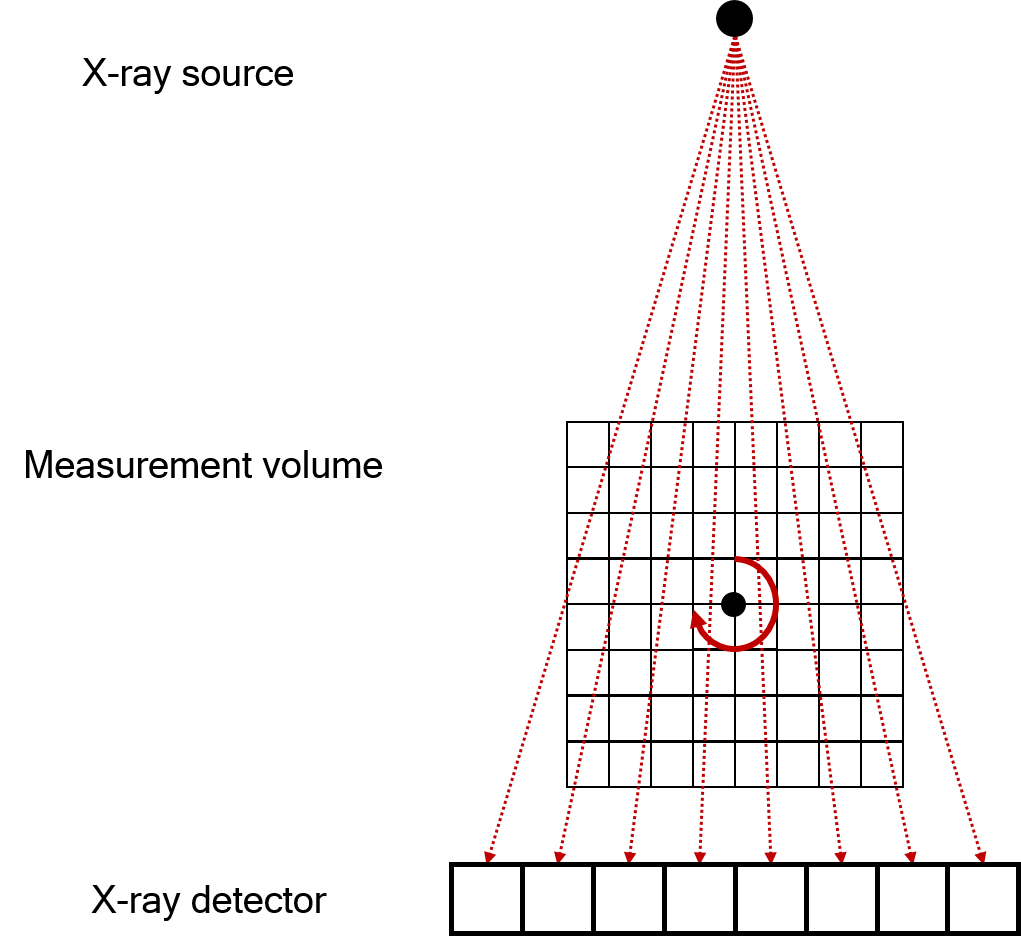
Fan beam geometry#
Cone-beam geometry#
A single point-like X-ray source emits a cone beam onto 2D detector array. Cone-beam geometry is mainly used in lab-based CT instruments. Depending on where the sample is placed between the source and the detector one can achieve a different magnification factor \(F\):
where \(r_1\) and \(r_2\) are the distance from the source to the center of the sample and the distance from the center of the sample to the detector, respectively.
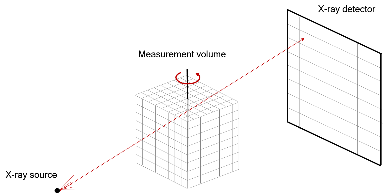
Cone beam geometry#
Multi channel data#
CIL is designed to work with 4D data.
Both AcquisitionGeometry, AcquisitionData and ImageGeometry, ImageData
can be defined for multi-channel (spectral/time) CT data using channels attribute.
Block Framework#
The block framework allows writing more advanced `optimisation problems`_. Consider the typical Tikhonov regularisation:
where,
\(A\) is the projection operator
\(b\) is the acquired data
\(u\) is the unknown image to be solved for
\(\alpha\) is the regularisation parameter
\(L\) is a regularisation operator
The first term measures the fidelity of the solution to the data. The second term measures the fidelity to the prior knowledge we have imposed on the system, operator \(L\).
This can be re-written equivalently in the block matrix form:
With the definitions:
\(\tilde{A} = \binom{A}{\alpha L}\)
\(\tilde{b} = \binom{b}{0}\)
this can now be recognised as a least squares problem which can be solved by any algorithm in the cil.optimisation
which can solve least squares problem, e.g. CGLS.
To be able to express our optimisation problems in the matrix form above, we developed the so-called,
Block Framework comprising 4 main actors: BlockGeometry, BlockDataContainer,
BlockFunction and BlockOperator.