Processors#
This module allows the user to manipulate or pre-process their data.
Data Manipulation#
These processors can be used on ImageData or AcquisitionData objects.
Data Slicer#
- class cil.processors.Slicer(roi=None)[source]#
This creates a Slicer processor.
The processor will crop the data, and then return every n input pixels along a dimension from the starting index.
The output will be a data container with the data, and geometry updated to reflect the operation.
- Parameters:
roi (dict) –
The region-of-interest to slice {‘axis_name1’:(start,stop,step), ‘axis_name2’:(start,stop,step)} The key being the axis name to apply the processor to, the value holding a tuple containing the ROI description
Start: Starting index of input data. Must be an integer, or None defaults to index 0. Stop: Stopping index of input data. Must be an integer, or None defaults to index N. Step: Number of pixels to average together. Must be an integer or None defaults to 1.
Example
>>> from cil.processors import Slicer
>>> roi = {'horizontal':(10,-10,2),'vertical':(10,-10,2)}
>>> processor = Slicer(roi)
>>> processor.set_input(data)
>>> data_sliced= processor.get_output()
Example
>>> from cil.processors import Slicer
>>> roi = {'horizontal':(None,None,2),'vertical':(None,None,2)}
>>> processor = Slicer(roi)
>>> processor.set_input(data.geometry)
>>> geometry_sliced = processor.get_output()
Note
The indices provided are start inclusive, stop exclusive.
All elements along a dimension will be included if the axis does not appear in the roi dictionary, or if passed as {‘axis_name’,-1}
If only one number is provided, then it is interpreted as Stop. i.e. {‘axis_name1’:(stop)} If two numbers are provided, then they are interpreted as Start and Stop i.e. {‘axis_name1’:(start, stop)}
Negative indexing can be used to specify the index. i.e. {‘axis_name1’:(10, -10)} will crop the dimension symmetrically
If Stop - Start is not multiple of Step, then the resulted dimension will have (Stop - Start) // Step elements, i.e. (Stop - Start) % Step elements will be ignored
- set_input(dataset)[source]#
Set the input data or geometry to the processor
- Parameters:
dataset (DataContainer, Geometry) – The input DataContainer or Geometry
- process(out=None)[source]#
Processes the input data
- Parameters:
out (ImageData, AcquisitionData, DataContainer, optional) – Fills the referenced DataContainer with the processed output and suppresses the return
- Returns:
The downsampled output is returned. Depending on the input type this may be: ImageData, AcquisitionData, DataContainer, ImageGeometry, AcquisitionGeometry
- Return type:
- get_output(out=None)#
Runs the configured processor and returns the processed data
- Parameters:
out (DataContainer, optional) – Fills the referenced DataContainer with the processed data
- Returns:
The processed data
- Return type:
Data Binner#
- class cil.processors.Binner(roi=None, accelerated=True)[source]#
This creates a Binner processor.
The processor will crop the data, and then average together n input pixels along a dimension from the starting index.
The output will be a data container with the data, and geometry updated to reflect the operation.
- Parameters:
roi (dict) –
The region-of-interest to bin {‘axis_name1’:(start,stop,step), ‘axis_name2’:(start,stop,step)} The key being the axis name to apply the processor to, the value holding a tuple containing the ROI description
Start: Starting index of input data. Must be an integer, or None defaults to index 0. Stop: Stopping index of input data. Must be an integer, or None defaults to index N. Step: Number of pixels to average together. Must be an integer or None defaults to 1.
accelerated (boolean, default=True) – Uses the CIL accelerated backend if True, numpy if False.
Example
>>> from cil.processors import Binner
>>> roi = {'horizontal':(10,-10,2),'vertical':(10,-10,2)}
>>> processor = Binner(roi)
>>> processor.set_input(data)
>>> data_binned = processor.get_output()
Example
>>> from cil.processors import Binner
>>> roi = {'horizontal':(None,None,2),'vertical':(None,None,2)}
>>> processor = Binner(roi)
>>> processor.set_input(data.geometry)
>>> geometry_binned = processor.get_output()
Note
The indices provided are start inclusive, stop exclusive.
All elements along a dimension will be included if the axis does not appear in the roi dictionary, or if passed as {‘axis_name’,-1}
If only one number is provided, then it is interpreted as Stop. i.e. {‘axis_name1’:(stop)} If two numbers are provided, then they are interpreted as Start and Stop i.e. {‘axis_name1’:(start, stop)}
Negative indexing can be used to specify the index. i.e. {‘axis_name1’:(10, -10)} will crop the dimension symmetrically
If Stop - Start is not multiple of Step, then the resulted dimension will have (Stop - Start) // Step elements, i.e. (Stop - Start) % Step elements will be ignored
- get_output(out=None)#
Runs the configured processor and returns the processed data
- Parameters:
out (DataContainer, optional) – Fills the referenced DataContainer with the processed data
- Returns:
The processed data
- Return type:
- process(out=None)#
Processes the input data
- Parameters:
out (ImageData, AcquisitionData, DataContainer, optional) – Fills the referenced DataContainer with the processed output and suppresses the return
- Returns:
The downsampled output is returned. Depending on the input type this may be: ImageData, AcquisitionData, DataContainer, ImageGeometry, AcquisitionGeometry
- Return type:
- set_input(dataset)#
Set the input data or geometry to the processor
- Parameters:
dataset (DataContainer, Geometry) – The input DataContainer or Geometry
Data Padder#
- class cil.processors.Padder(mode='constant', pad_width=None, pad_values=0)[source]#
Processor to pad an array with a border, wrapping numpy.pad. See https://numpy.org/doc/stable/reference/generated/numpy.pad.html
It is recommended to use the static methods to configure your Padder object rather than initialising this class directly. See examples for details.
- Parameters:
mode (str) – The method used to populate the border data. Accepts: ‘constant’, ‘edge’, ‘linear_ramp’, ‘reflect’, ‘symmetric’, ‘wrap’
pad_width (int, tuple, dict) – The size of the border along each axis, see usage notes
pad_values (float, tuple, dict, default=0.0) – The additional values needed by some of the modes
Notes
- pad_width behaviour (number of pixels):
int: Each axis will be padded with a border of this size
tuple(int, int): Each axis will be padded with an asymmetric border i.e. (before, after)
dict: Specified axes will be padded: e.g. {‘horizontal’:(8, 23), ‘vertical’: 10}
- pad_values behaviour:
float: Each border will use this value
tuple(float, float): Each value will be used asymmetrically for each axis i.e. (before, after)
dict: Specified axes and values: e.g. {‘horizontal’:(8, 23), ‘channel’:5}
If padding angles the angular values assigned to the padded axis will be extrapolated from the first two, and the last two angles in geometry.angles. The user should ensure the output is as expected.
Example
>>> processor = Padder.edge(pad_width=1)
>>> processor.set_input(data)
>>> data_padded = processor.get_output()
>>> print(data.array)
[[0. 1. 2.]
[3. 4. 5.]
[6. 7. 8.]]
>>> print(data_padded.array)
[[0. 0. 1. 2. 2.]
[0. 0. 1. 2. 2.]
[3. 3. 4. 5. 5.]
[6. 6. 7. 8. 8.]
[6. 6. 7. 8. 8.]]
Example
>>> processor = Padder.constant(pad_width={'horizontal_y':(1,1),'horizontal_x':(1,2)}, constant_values=(-1.0, 1.0))
>>> processor.set_input(data)
>>> data_padded = processor.get_output()
>>> print(data.array)
[[0. 1. 2.]
[3. 4. 5.]
[6. 7. 8.]]
>>> print(data_padded.array)
[[-1. -1. -1. -1.  1.  1.]
[-1.  0.  1.  2.  1.  1.]
[-1.  3.  4.  5.  1.  1.]
[-1.  6.  7.  8.  1.  1.]
[-1.  1.  1.  1.  1.  1.]
- static constant(pad_width=None, constant_values=0.0)[source]#
Padder processor wrapping numpy.pad with mode constant.
Pads the data with a constant value border. Pads in all spatial dimensions unless a dictionary is passed to either pad_width or constant_values
- Parameters:
pad_width (int, tuple, dict) – The size of the border along each axis, see usage notes
constant_values (float, tuple, dict, default=0.0) – The value of the border, see usage notes
Notes
- pad_width behaviour (number of pixels):
int: Each axis will be padded with a border of this size
tuple(int, int): Each axis will be padded with an asymmetric border i.e. (before, after)
dict: Specified axes will be padded: e.g. {‘horizontal’:(8, 23), ‘vertical’: 10}
- constant_values behaviour (value of pixels):
float: Each border will be set to this value
tuple(float, float): Each border value will be used asymmetrically for each axis i.e. (before, after)
dict: Specified axes and values: e.g. {‘horizontal’:(8, 23), ‘channel’:5}
If padding angles the angular values assigned to the padded axis will be extrapolated from the first two, and the last two angles in geometry.angles. The user should ensure the output is as expected.
Example
>>> processor = Padder.constant(pad_width=1, constant_values=0.0)
>>> processor.set_input(data)
>>> data_padded = processor.get_output()
>>> print(data.array)
[[0. 1. 2.]
[3. 4. 5.]
[6. 7. 8.]]
>>> print(data_padded.array)
[[0. 0. 0. 0. 0.]
[0. 0. 1. 2. 0.]
[0. 3. 4. 5. 0.]
[0. 6. 7. 8. 0.]
[0. 0. 0. 0. 0.]]
- static edge(pad_width=None)[source]#
Padder processor wrapping numpy.pad with mode edge.
Pads the data by extending the edge values in to the border. Pads in all spatial dimensions unless a dictionary is passed to pad_width.
- pad_width: int, tuple, dict
The size of the border along each axis, see usage notes
Notes
- pad_width behaviour (number of pixels):
int: Each axis will be padded with a border of this size
tuple(int, int): Each axis will be padded with an asymmetric border i.e. (before, after)
dict: Specified axes will be padded: e.g. {‘horizontal’:(8, 23), ‘vertical’: 10}
If padding angles the angular values assigned to the padded axis will be extrapolated from the first two, and the last two angles in geometry.angles. The user should ensure the output is as expected.
Example
>>> processor = Padder.edge(pad_width=1)
>>> processor.set_input(data)
>>> data_padded = processor.get_output()
>>> print(data.array)
[[0. 1. 2.]
[3. 4. 5.]
[6. 7. 8.]]
>>> print(data_padded.array)
[[0. 0. 1. 2. 2.]
[0. 0. 1. 2. 2.]
[3. 3. 4. 5. 5.]
[6. 6. 7. 8. 8.]
[6. 6. 7. 8. 8.]]
- static linear_ramp(pad_width=None, end_values=0.0)[source]#
Padder processor wrapping numpy.pad with mode linear_ramp
Pads the data with values calculated from a linear ramp between the array edge value and the set end_value. Pads in all spatial dimensions unless a dictionary is passed to either pad_width or constant_values
- pad_width: int, tuple, dict
The size of the border along each axis, see usage notes
- end_values: float, tuple, dict, default=0.0
The target value of the linear_ramp, see usage notes
Notes
- pad_width behaviour (number of pixels):
int: Each axis will be padded with a border of this size
tuple(int, int): Each axis will be padded with an asymmetric border i.e. (before, after)
dict: Specified axes will be padded: e.g. {‘horizontal’:(8, 23), ‘vertical’: 10}
- end_values behaviour:
float: Each border will use this end value
tuple(float, float): Each border end value will be used asymmetrically for each axis i.e. (before, after)
dict: Specified axes and end values: e.g. {‘horizontal’:(8, 23), ‘channel’:5}
If padding angles the angular values assigned to the padded axis will be extrapolated from the first two, and the last two angles in geometry.angles. The user should ensure the output is as expected.
Example
>>> processor = Padder.linear_ramp(pad_width=2, end_values=0.0)
>>> processor.set_input(data)
>>> data_padded = processor.get_output()
>>> print(data.array)
[[0. 1. 2.]
[3. 4. 5.]
[6. 7. 8.]]
>>> print(data_padded.array)
[[0.  0.  0.  0.  0.  0.  0. ]
[0.  0.  0.  0.5 1.  0.5 0. ]
[0.  0.  0.  1.  2.  1.  0. ]
[0.  1.5 3.  4.  5.  2.5 0. ]
[0.  3.  6.  7.  8.  4.  0. ]
[0.  1.5 3.  3.5 4.  2.  0. ]
[0.  0.  0.  0.  0.  0.  0. ]]
- static reflect(pad_width=None)[source]#
Padder processor wrapping numpy.pad with mode reflect.
Pads with the reflection of the data mirrored along first and last values each axis. Pads in all spatial dimensions unless a dictionary is passed to pad_width.
- pad_width: int, tuple, dict
The size of the border along each axis, see usage notes
Notes
- pad_width behaviour (number of pixels):
int: Each axis will be padded with a border of this size
tuple(int, int): Each axis will be padded with an asymmetric border i.e. (before, after)
dict: Specified axes will be padded: e.g. {‘horizontal’:(8, 23), ‘vertical’: 10}
If padding angles the angular values assigned to the padded axis will be extrapolated from the first two, and the last two angles in geometry.angles. The user should ensure the output is as expected.
Example
>>> processor = Padder.reflect(pad_width=1)
>>> processor.set_input(data)
>>> data_padded = processor.get_output()
>>> print(data.array)
[[0. 1. 2.]
[3. 4. 5.]
[6. 7. 8.]]
>>> print(data_padded.array)
[[4. 3. 4. 5. 4.]
[1. 0. 1. 2. 1.]
[4. 3. 4. 5. 4.]
[7. 6. 7. 8. 7.]
[4. 3. 4. 5. 4.]]
- static symmetric(pad_width=None)[source]#
Padder processor wrapping numpy.pad with mode symmetric.
Pads with the reflection of the data mirrored along the edge of the array. Pads in all spatial dimensions unless a dictionary is passed to pad_width.
- Parameters:
pad_width (int, tuple, dict) – The size of the border along each axis
Notes
- pad_width behaviour (number of pixels):
int: Each axis will be padded with a border of this size
tuple(int, int): Each axis will be padded with an asymmetric border i.e. (before, after)
dict: Specified axes will be padded: e.g. {‘horizontal’:(8, 23), ‘vertical’: 10}
If padding angles the angular values assigned to the padded axis will be extrapolated from the first two, and the last two angles in geometry.angles. The user should ensure the output is as expected.
Example
>>> processor = Padder.symmetric(pad_width=1)
>>> processor.set_input(data)
>>> data_padded = processor.get_output()
>>> print(data.array)
[[0. 1. 2.]
[3. 4. 5.]
[6. 7. 8.]]
>>> print(data_padded.array)
[[0. 0. 1. 2. 2.]
[0. 0. 1. 2. 2.]
[3. 3. 4. 5. 5.]
[6. 6. 7. 8. 8.]
[6. 6. 7. 8. 8.]]
- static wrap(pad_width=None)[source]#
Padder processor wrapping numpy.pad with mode wrap.
Pads with the wrap of the vector along the axis. The first values are used to pad the end and the end values are used to pad the beginning. Pads in all spatial dimensions unless a dictionary is passed to pad_width.
- Parameters:
pad_width (int, tuple, dict) – The size of the border along each axis
Notes
- pad_width behaviour (number of pixels):
int: Each axis will be padded with a border of this size
tuple(int, int): Each axis will be padded with an asymmetric border i.e. (before, after)
dict: Specified axes will be padded: e.g. {‘horizontal’:(8, 23), ‘vertical’: 10}
If padding angles the angular values assigned to the padded axis will be extrapolated from the first two, and the last two angles in geometry.angles. The user should ensure the output is as expected.
Example
>>> processor = Padder.wrap(pad_width=1)
>>> processor.set_input(data)
>>> data_padded = processor.get_output()
>>> print(data.array)
[[0. 1. 2.]
[3. 4. 5.]
[6. 7. 8.]]
>>> print(data_padded.array)
[[8. 6. 7. 8. 6.]
[2. 0. 1. 2. 0.]
[5. 3. 4. 5. 3.]
[8. 6. 7. 8. 6.]
[2. 0. 1. 2. 0.]]
- set_input(dataset)[source]#
Set the input data to the processor
- Parameters:
dataset (DataContainer, Geometry) – The input DataContainer
- get_output(out=None)#
Runs the configured processor and returns the processed data
- Parameters:
out (DataContainer, optional) – Fills the referenced DataContainer with the processed data
- Returns:
The processed data
- Return type:
Mask Generator from Data#
- class cil.processors.MaskGenerator(mode='special_values', threshold_value=(None, None), quantiles=(None, None), threshold_factor=3, window=5, axis=None)[source]#
Processor to detect outliers and return a mask with 0 where outliers were detected, and 1 for other pixels. Please use the desiried method to configure a processor for your needs.
- static special_values(nan=True, inf=True)[source]#
This creates a MaskGenerator processor which generates a mask for inf and/or nan values.
- Parameters:
nan (bool, default=True) – mask NaN values
inf (bool, default=True) – mask INF values
- static threshold(min_val=None, max_val=None)[source]#
This creates a MaskGenerator processor which generates a mask for values outside boundaries
- Parameters:
min_val (float, default=None) – lower boundary
max_val (float, default=None) – upper boundary
- static quantile(min_quantile=None, max_quantile=None)[source]#
This creates a MaskGenerator processor which generates a mask for values outside boundaries
- Parameters:
min_quantile (float, default=None) – lower quantile, 0-1
max_quantile (float, default=None) – upper quantile, 0-1
- static mean(axis=None, threshold_factor=3, window=None)[source]#
This creates a MaskGenerator processor which generates a mask for values outside a multiple of standard-devaiations from the mean.
abs(A - mean(A)) < threshold_factor * std(A).
- Parameters:
threshold_factor (float, default=3) – scale factor of standard-deviations to use as threshold
axis (int, string) – specify axis as int or from ‘dimension_labels’ to calculate mean. If no axis is specified then operates over flattened array.
window (int, default=None) – specify number of pixels to use in calculation of a rolling mean
- static median(axis=None, threshold_factor=3, window=None)[source]#
This creates a MaskGenerator processor which generates a mask for values outside a multiple of median absolute deviation (MAD) from the mean.
abs(A - median(A)) < threshold_factor * MAD(A), MAD = c*median(abs(A-median(A))) where c=-1/(sqrt(2)*erfcinv(3/2))
- Parameters:
threshold_factor (float, default=3) – scale factor of MAD to use as threshold
axis (int, string) – specify axis as int or from ‘dimension_labels’ to calculate mean. If no axis is specified then operates over flattened array.
window (int, default=None) – specify number of pixels to use in calculation of a rolling median
- get_output(out=None)#
Runs the configured processor and returns the processed data
- Parameters:
out (DataContainer, optional) – Fills the referenced DataContainer with the processed data
- Returns:
The processed data
- Return type:
- set_input(dataset)#
Set the input data to the processor
- Parameters:
input (DataContainer) – The input DataContainer
Data Masking#
- class cil.processors.Masker(mask=None, mode='value', value=0, axis=None, method='linear')[source]#
Processor to fill missing values provided by mask. Please use the desired method to configure a processor for your needs.
- Parameters:
mask (DataContainer, ImageData, AcquisitionData, numpy.ndarray) – A boolean array with the same dimensions as input, where ‘False’ represents masked values. Alternatively an integer array where 0 represents masked values, and any other value represents unmasked values. Mask can be generated using ‘MaskGenerator’ processor to identify outliers.
mode ({'value', 'mean', 'median', 'interpolate'}, default='value') – The method to fill in missing values
value (float, default=0) – Substitute all outliers with a specific value if method=’value’, otherwise discarded.
axis (str or int) – Specify axis as int or from ‘dimension_labels’ to calculate mean, median or interpolation (depending on mode) along that axis. If you specify an axis, values are collected to calculate the missing pixel by varying the index of that axis, leaving all other indices fixed.
method ({'linear', 'nearest', 'zeros', 'linear', 'quadratic', 'cubic', 'previous', 'next'}, default='linear') – Interpolation method to use.
- static value(mask=None, value=0)[source]#
Returns a Masker that sets the masked values of the input data to the requested value.
- Parameters:
mask (DataContainer, ImageData, AcquisitionData, numpy.ndarray) – A boolean array with the same dimensions as input, where ‘False’ represents masked values. Alternatively an integer array where 0 represents masked values, and any other value represents unmasked values. Mask can be generated using ‘MaskGenerator’ processor to identify outliers.
value (float, default=0) – Values to be assigned to missing elements
- Return type:
Masker processor
- static mean(mask=None, axis=None)[source]#
Returns a Masker that sets the masked values of the input data to the mean of the unmasked values across the array or along the specified axis.
- Parameters:
mask (DataContainer, ImageData, AcquisitionData, numpy.ndarray) – A boolean array with the same dimensions as input, where ‘False’ represents masked values. Alternatively an integer array where 0 represents masked values, and any other value represents unmasked values. Mask can be generated using ‘MaskGenerator’ processor to identify outliers.
axis (str, int) – Axis along which the means are computed. Specified by an int or from ‘dimension_labels’. If you specify an axis, values are collected to calculate the missing pixel by varying the index of that axis, leaving all other indices fixed.
- Return type:
Masker processor
- static median(mask=None, axis=None)[source]#
Returns a Masker that sets the masked values of the input data to the median of the unmasked values across the array or along the specified axis.
- Parameters:
mask (DataContainer, ImageData, AcquisitionData, numpy.ndarray) – A boolean array with the same dimensions as input, where ‘False’ represents masked values. Alternatively an integer array where 0 represents masked values, and any other value represents unmasked values. Mask can be generated using ‘MaskGenerator’ processor to identify outliers.
axis (str, int) –
Axis along which the medians are computed. Specified by an int or from ‘dimension_labels’. If you specify an axis, values are collected to calculate the missing pixel by varying the index of that axis,
leaving all other indices fixed.
- Return type:
Masker processor
- static interpolate(mask=None, axis=None, method='linear')[source]#
Returns a Masker that operates over the specified axis and uses 1D interpolation over remaining flattened array to fill in missing values.
- Parameters:
mask (DataContainer, ImageData, AcquisitionData, numpy.ndarray) – A boolean array with the same dimensions as input, where ‘False’ represents masked values. Alternatively an integer array where 0 represents masked values, and any other value represents unmasked values. Mask can be generated using ‘MaskGenerator’ processor to identify outliers.
axis (str, int) – Specify axis as int or from ‘dimension_labels’ to loop over and perform 1D interpolation.
method ({'linear', 'nearest', 'zeros', 'linear', 'quadratic', 'cubic', 'previous', 'next'}, default='linear') – Interpolation method to use.
- Return type:
Masker processor
- get_output(out=None)#
Runs the configured processor and returns the processed data
- Parameters:
out (DataContainer, optional) – Fills the referenced DataContainer with the processed data
- Returns:
The processed data
- Return type:
- set_input(dataset)#
Set the input data to the processor
- Parameters:
input (DataContainer) – The input DataContainer
Pre-processors#
These processors can be used with AcquisitionData objects
Centre Of Rotation Corrector#
In the ideal alignment of a CT instrument, the projection of the axis of rotation onto the detector coincides with the vertical midline of the detector. In practice this is hard to achieve due to misalignments and/or kinematic errors in positioning of CT instrument components. A slight offset of the center of rotation with respect to the theoretical position will contribute to the loss of resolution; in more severe cases, it will cause severe artifacts in the reconstructed volume (double-borders).
CentreOfRotationCorrector can be used to estimate the offset of center of rotation from the data.
CentreOfRotationCorrector supports both parallel and cone-beam geometry with 2 different algorithms:
Cross-correlation, is suitable for single slice parallel-beam geometry. It requires two projections 180 degree apart.
Image sharpness method, which maximising the sharpness of a reconstructed slice. It can be used on single
slice parallel-beam, and centre-slice of cone-beam geometry. For use only with datasets that can be reconstructed with FBP/FDK.
- class cil.processors.CentreOfRotationCorrector(**attributes)[source]#
This class contains methods to create a CentreOfRotationCorrector processor using the desired algorithm.
- static xcorrelation(slice_index='centre', projection_index=0, ang_tol=0.1)[source]#
This creates a CentreOfRotationCorrector processor using the cross-correlation algorithm.
For use on parallel-beam geometry it requires two projections 180 degree apart.
- Parameters:
slice_index (int or str, optional) – An integer defining the vertical slice to run the algorithm on or string=’centre’ specifying the central slice should be used (default is ‘centre’)
projection_index (int or list/tuple of ints, optional) – An integer defining the index of the first projection the cross correlation algorithm will use, where the second projection is chosen as the projection closest to 180 degrees from this. Or a list/tuple of ints specifying the two indices to be used for cross correlation (default is 0)
ang_tol (float, optional) – The angular tolerance in degrees between the two input projections 180 degree gap (default is 0.1)
Example
>>> from cil.processors import CentreOfRotationCorrector
>>> processor = CentreOfRotationCorrector.xcorrelation('centre')
>>> processor.set_input(data)
>>> data_centred = processor.get_ouput()
Example
>>> from cil.processors import CentreOfRotationCorrector
>>> processor = CentreOfRotationCorrector.xcorrelation(slice_index=120)
>>> processor.set_input(data)
>>> processor.get_ouput(out=data)
Example
>>> from cil.processors import CentreOfRotationCorrector
>>> import logging
>>> logging.basicConfig(level=logging.WARNING)
>>> cil_log_level = logging.getLogger('cil.processors')
>>> cil_log_level.setLevel(logging.DEBUG)
>>> processor = CentreOfRotationCorrector.xcorrelation(slice_index=120)
>>> processor.set_input(data)
>>> data_centred = processor.get_output()
Note
setting logging to ‘debug’ will give you more information about the algorithm progress
- static image_sharpness(slice_index='centre', backend='tigre', tolerance=0.005, search_range=None, initial_binning=None)[source]#
This creates a CentreOfRotationCorrector processor.
The processor will find the centre offset by maximising the sharpness of a reconstructed slice.
Can be used on single slice parallel-beam, and centre slice cone beam geometry. For use only with datasets that can be reconstructed with FBP/FDK.
- Parameters:
slice_index (int, str, default='centre') – An integer defining the vertical slice to run the algorithm on. The special case slice ‘centre’ is the default.
backend ({'tigre', 'astra'}) – The backend to use for the reconstruction
tolerance (float, default=0.005) – The tolerance of the fit in pixels, the default is 1/200 of a pixel. This is a stopping criteria, not a statement of accuracy of the algorithm.
search_range (int) – The range in pixels to search either side of the panel centre. If None a quarter of the width of the panel is used.
initial_binning (int) – The size of the bins for the initial search. If None will bin the image to a step corresponding to <128 pixels. The fine search will be on unbinned data.
Example
from cil.processors import CentreOfRotationCorrector
processor = CentreOfRotationCorrector.image_sharpness(‘centre’, ‘tigre’) processor.set_input(data) data_centred = processor.get_output()
Example
from cil.processors import CentreOfRotationCorrector
processor = CentreOfRotationCorrector.image_sharpness(slice_index=120, ‘astra’) processor.set_input(data) processor.get_output(out=data)
Note
For best results data should be 360deg which leads to blurring with incorrect geometry. This method is unreliable on half-scan data with ‘tuning-fork’ style artifacts.
- get_output(out=None)#
Runs the configured processor and returns the processed data
- Parameters:
out (DataContainer, optional) – Fills the referenced DataContainer with the processed data
- Returns:
The processed data
- Return type:
- set_input(dataset)#
Set the input data to the processor
- Parameters:
input (DataContainer) – The input DataContainer
Data Normaliser#
- class cil.processors.Normaliser(flat_field=None, dark_field=None, tolerance=1e-05)[source]#
This processor can be used to normalise data with flat-field and dark-field images.
The dark-field image is used to remove the offset from the input data, and the flat-field image is used to scale the data.
The normalisation is done as follows:
\[\text{output} = \frac{\text{input} - \text{offset}}{\text{scale} - \text{offset}}\]where \(\text{input}\), \(\text{offset}\) and \(\text{scale}\) are the input, dark-field and flat-field images respectively.
The processor can be used in-place to reduce memory usage.
- Parameters:
flat_field (numpy.ndarray, optional) – The flat field image. It must have the same shape as a single projection.
dark_field (numpy.ndarray, optional) – The dark field image. It must have the same shape as a single projection.
tolerance (float, optional) – The value to substitute for output values where division by zero occurs.
Examples
Basic usage with flat and dark fields:
>>> from cil.processors import Normaliser
>>> normaliser = Normaliser(flat_field, dark_field)
>>> normaliser.set_input(data)
>>> normalised_data = normaliser.get_output()
In-place usage:
>>> from cil.processors import Normaliser
>>> normaliser = Normaliser(flat_field, dark_field)
>>> normaliser.set_input(data)
>>> normaliser.get_output(out=data)
- static estimate_normalised_error(projection, flat, dark, delta_flat, delta_dark)[source]#
returns the estimated relative error of the normalised projection
n = (projection - dark) / (flat - dark) Dn/n = (flat-dark + projection-dark)/((flat-dark)*(projection-dark))*(Df/f + Dd/d)
- get_output(out=None)#
Runs the configured processor and returns the processed data
- Parameters:
out (DataContainer, optional) – Fills the referenced DataContainer with the processed data
- Returns:
The processed data
- Return type:
- set_input(dataset)#
Set the input data to the processor
- Parameters:
input (DataContainer) – The input DataContainer
Flux Normaliser#
- class cil.processors.FluxNormaliser(flux=None, roi=None, target='mean', accelerated=True)[source]#
Flux normalisation based on float or region of interest
This processor reads in an AcquisitionData and normalises it by flux from a float or array of float values, or the mean flux in a region of interest. Each projection is divided by its flux value and multiplied by the target.
Parameters:#
- flux: float or list of floats, optional
Array of floats that describe the variation in brightness of the unobstructed beam between projections. Must have length equal to the number of projections in the dataset, or be a single float. If flux=None, calculate flux from the roi.
- roi: dict, optional
Dictionary describing the region of interest containing the background in the image from which to extract the flux. The roi is specified as {‘horizontal’:(start,stop), ‘vertical’:(start,stop)}. If an axis is not specified in the roi dictionary, the full range will be used.
- target: {‘mean’, ‘first’, ‘last’} or float, default=’mean’
The target of the normalised data. If string the data is scaled by the ‘mean’, ‘first’ or ‘last’ flux value. If float, the data is scaled by the float value. Default is ‘mean’
- accelerated: bool, optional
Specify whether to use multi-threading using numba. Default is True
Returns:#
Output: AcquisitionData normalised by flux
Example
This example passes the flux as a list the same size as the data, and specifies the target=’first’ which scales all projections to the first flux value 0.9 >>> from cil.processors import FluxNormaliser >>> processor = FluxNormaliser(flux=[0.9, 1.0, 1.1, 0.8], target=’first’) >>> processor.set_input(data) >>> data_norm = processor.get_output()
Example
This example calculates the flux from a region of interest for each projection and scales all projections to the mean flux >>> from cil.processors import FluxNormaliser >>> processor = FluxNormaliser(roi={‘horizontal’:(5, 15)}, target=’mean’) >>> processor.set_input(data) >>> data_norm = processor.get_output()
Note
The roi indices provided are start inclusive, stop exclusive. All elements along a dimension will be included if the axis does not appear in the roi dictionary
- preview_configuration(projection_index=None, channel=None, log=False, **kwargs)[source]#
Preview the FluxNormalisation processor configuration for roi mode. Plots the region of interest on the image and the mean, maximum and minimum intensity in the roi.
Requires matplotlib (or matplotlib-base) to be installed
Parameters:#
- projection_index: int, optional
Index of the projection to plot, default=None displays the data with the minimum and maximum pixel values in the roi. For 2D data, the roi is plotted on the sinogram.
- channel: int, optional
The channel to plot, default=None displays the central channel if the data has channels
- log: bool, default=False
If True, plot the image with a log scale, default is False
- **kwargs:
- angle: int, optional
Deprecated alias for projection_index. Use projection_index instead.
Returns:#
- matplotlib.figure.Figure
The figure object created to plot the configuration
- get_output(out=None)#
Runs the configured processor and returns the processed data
- Parameters:
out (DataContainer, optional) – Fills the referenced DataContainer with the processed data
- Returns:
The processed data
- Return type:
- set_input(dataset)#
Set the input data to the processor
- Parameters:
input (DataContainer) – The input DataContainer
Transmission to Absorption Converter#
- class cil.processors.TransmissionAbsorptionConverter(min_intensity=0.0, white_level=1.0, accelerated=True)[source]#
Processor to convert from transmission measurements to absorption based on the Beer-Lambert law, by: - dividing by white_level, - clipping data to min_intensity (any values below min intensity are set to min_intensity) - taking the logarithm and multiplying by minus 1. If the data contains zero or negative values, inf or NaN values will be present in the output.
Parameters:#
- min_intensity: float, default=0.0
Clips data below this value to ensure log is taken of positive numbers only.
- white_level: float, default=1.0
A float defining incidence intensity in the Beer-Lambert law.
- accelerated: bool, default=True
Specify whether to use multi-threading using numba.
Returns:#
AcquisitionData, ImageData or DataContainer depending on input data type, return is suppressed if ‘out’ is passed
Notes:#
If it’s unknown whether the data contains zero or negative values, it’s recommended to set min_intensity to a small positive value.
- get_output(out=None)#
Runs the configured processor and returns the processed data
- Parameters:
out (DataContainer, optional) – Fills the referenced DataContainer with the processed data
- Returns:
The processed data
- Return type:
- set_input(dataset)#
Set the input data to the processor
- Parameters:
input (DataContainer) – The input DataContainer
Absorption to Transmission Converter#
- class cil.processors.AbsorptionTransmissionConverter(white_level=1)[source]#
Processor to convert from absorption measurements to transmission
- Parameters:
white_level (float, optional) – A float defining incidence intensity in the Beer-Lambert law.
- Returns:
returns AcquisitionData, ImageData or DataContainer depending on input data type
- Return type:
Processor first multiplies data by -1, then calculates exponent and scales result by white_level (default=1)
- get_output(out=None)#
Runs the configured processor and returns the processed data
- Parameters:
out (DataContainer, optional) – Fills the referenced DataContainer with the processed data
- Returns:
The processed data
- Return type:
- set_input(dataset)#
Set the input data to the processor
- Parameters:
input (DataContainer) – The input DataContainer
Ring Remover#
- class cil.processors.RingRemover(decNum=4, wname='db10', sigma=1.5, info=True)[source]#
RingRemover Processor: Removes vertical stripes from a DataContainer(ImageData/AcquisitionData) using the algorithm in https://doi.org/10.1364/OE.17.008567
- Parameters:
decNum (int) – Number of wavelet decompositions - increasing the number of decompositions, increases the strength of the ring removal but can alter the profile of the data
wname (str) – Name of wavelet filter from pywt e.g. ‘db1’ – ‘db35’, ‘haar’ - increasing the wavelet filter increases the strength of the ring removal, but also increases the computational effort
sigma (float) – Damping parameter in Fourier space - increasing sigma, increases the size of artefacts which can be removed
info (boolean) – Flag to enable print of ring remover end message
- Returns:
Corrected ImageData/AcquisitionData 2D, 3D, multi-spectral 2D, multi-spectral 3D
- Return type:
- get_output(out=None)#
Runs the configured processor and returns the processed data
- Parameters:
out (DataContainer, optional) – Fills the referenced DataContainer with the processed data
- Returns:
The processed data
- Return type:
- set_input(dataset)#
Set the input data to the processor
- Parameters:
input (DataContainer) – The input DataContainer
Paganin Processor#
- class cil.processors.PaganinProcessor(delta=1, beta=0.01, energy=40000, energy_units='eV', full_retrieval=True, filter_type='paganin_method', pad=0, return_units='cm')[source]#
Processor to retrieve quantitative information from phase contrast images using the Paganin phase retrieval algorithm described in [1]
- Parameters:
delta (float (optional)) – Real part of the deviation of the material refractive index from 1, where refractive index \(n = (1 - \delta) + i \beta\) energy- dependent refractive index information for x-ray wavelengths can be found at [2], default is 1
beta (float (optional)) – Complex part of the material refractive index, where refractive index \(n = (1 - \delta) + i \beta\) energy-dependent refractive index information for x-ray wavelengths can be found at [2], default is 1e-2
energy (float (optional)) – Energy of the incident photon, default is 40000
energy_units (string (optional)) – Energy units, default is ‘eV’
full_retrieval (bool, optional) – If True, perform the full phase retrieval and return the thickness. If False, return a filtered image, default is True
filter_type (string (optional)) – The form of the Paganin filter to use, either ‘paganin_method’ (default) or ‘generalised_paganin_method’ as described in [3]
pad (int (optional)) – Number of pixels to pad the image in Fourier space to reduce aliasing, default is 0
return_units (string (optional)) – The distance units to return the sample thickness in, must be one of ‘m’, ‘cm’, ‘mm’ or ‘um’. Only applies if full_retrieval=True (default is’cm’)
- Returns:
AcquisitionData corrected for phase effects, retrieved sample thickness or (if
full_retrieval=False) filtered data- Return type:
Example
>>> processor = PaganinProcessor(delta=5, beta=0.05, energy=18000)
>>> processor.set_input(data)
>>> thickness = processor.get_output()
Example
>>> processor = PaganinProcessor(delta=1,beta=10e2, full_retrieval=False)
>>> processor.set_input(data)
>>> filtered_image = processor.get_output()
Example
>>> processor = PaganinProcessor()
>>> processor.set_input(data)
>>> thickness = processor.get_output(override_filter={'alpha':10})
>>> phase_retrieved_image = thickness*processor.mu
Notes
This processor will work most efficiently using the cil data order with data.reorder(‘cil’)
Notes
This processor uses the phase retrieval algorithm described by Paganin et al. [1] to retrieve the sample thickness
\[T(x,y) = - \frac{1}{\mu}\ln\left (\mathcal{F}^{-1}\left (\frac{\mathcal{F}\left ( I_{norm}(x, y,z = \Delta) \right )}{1 + \alpha\left ( k_x^2 + k_y^2 \right )} \right )\right ),\]where
\(T\), is the sample thickness,
\(\mu = \frac{4\pi\beta}{\lambda}\) is the material linear attenuation coefficient where \(\beta\) is the complex part of the material refractive index [2] and \(\lambda=\frac{hc}{E}\) is the probe wavelength,
\(I_{norm}\) is the input image which is expected to be the normalised transmission data,
\(\Delta\) is the propagation distance. In cone-beam geometry, \(\Delta\) is scaled by the magnification \(M\) as described in [1],
\(\alpha = \frac{\Delta\delta}{\mu}\) is a parameter determining the strength of the filter to be applied in Fourier space where \(\delta\) is the real part of the deviation of the material refractive index from 1 [2].
\(k_x, k_y = \left ( \frac{2\pi p}{N_xW}, \frac{2\pi q}{N_yW} \right )\) where \(p\) and \(q\) are co-ordinates in a Fourier mesh in the range \(-N_x/2\) to \(N_x/2\) for an image with size \(N_x, N_y\) and pixel size \(W\). In cone-beam geometry, the pixel size is scaled by the magnification \(M\).
A generalised form of the Paganin phase retrieval method can be called using
filter_type='generalised_paganin_method', which uses the form of the algorithm described in [3]\[T(x,y) = -\frac{1}{\mu}\ln\left (\mathcal{F}^{-1}\left (\frac{ \mathcal{F}\left (I_{norm}(x, y,z = \Delta) \right )}{1 - \frac{2 \alpha}{W^2}\left ( \cos(Wk_x) + \cos(Wk_y) -2 \right )} \right ) \right )\]The phase retrieval is valid under the following assumptions
used with paraxial propagation-induced phase contrast images which
can be assumed to be single-material locally - using intensity data which has been flat field corrected - and under the assumption that the Fresnel number \(F_N = W^2/(\lambda\Delta) >> 1\)
To apply a filter to images using the Paganin method, call
full_retrieval=False. In this case the pre-scaling and conversion to absorption is not applied so the requirement to supply flat field corrected intensity data is relaxed,\[I_{filt} = \mathcal{F}^{-1}\left (\frac{\mathcal{F}\left ( I(x, y,z = \Delta) \right )} {1 - \alpha\left ( k_x^2 + k_y^2 \right )} \right )\]References
With thanks to colleagues at DTU for help with the initial implementation of the phase retrieval algorithm
- set_input(dataset)[source]#
Set the input data to the processor
- Parameters:
dataset (AcquisitionData) – The input AcquisitionData
- get_output(out=None, override_geometry=None, override_filter=None)[source]#
Function to get output from the PaganinProcessor
- Parameters:
out (DataContainer, optional) – Fills the referenced DataContainer with the processed data
override_geometry (dict, optional) – Geometry parameters to use in the phase retrieval if you want to over-ride values found in data.geometry. Specify parameters as a dictionary
{'parameter':value}where parameter is'magnification', 'propagation_distance'or'pixel_size'and value is the new value to use. Specify distance parameters in the same units asreturn_units(default is cm).override_filter (dict, optional) – Over-ride the filter parameters to use in the phase retrieval. Specify parameters as
{'parameter':value}where parameter is'delta', 'beta'or'alpha'and value is the new value to use.
- Returns:
AcquisitionData corrected for phase effects, retrieved sample thickness or (if
full_retrieval=False) filtered data- Return type:
Example
>>> processor = PaganinProcessor(delta=5, beta=0.05, energy=18000)
>>> processor.set_input(data)
>>> thickness = processor.get_output()
Example
>>> processor = PaganinProcessor(delta=1,beta=10e2,
full_retrieval=False)
>>> processor.set_input(data)
>>> filtered_image = processor.get_output()
Example
>>> processor = PaganinProcessor()
>>> processor.set_input(data)
>>> thickness = processor.get_output(override_filter={'alpha':10})
>>> phase_retrieved_image = thickness*processor.mu
Notes
If
'alpha'is specified in override_filter the new value will be used and delta will be ignored but beta will still be used to calculate \(\mu = \frac{4\pi\beta}{\lambda}\) which is used for scaling the thickness, therefore it is only recommended to specify alpha when also usingget_output(full_retrieval=False), or re-scaling the result by \(\mu\) e.g.thickness*processor.muIfalphais not specified, it will be calculated \(\frac{\Delta\delta\lambda}{4\pi\beta}\)
Laminography Geometry Corrector#
Laminography is a technique similar to tomography in which the rotation axis is tilted relative to the beam. This can be setup as below, by tilting the sample and rotation axis by an angle \(\phi\):
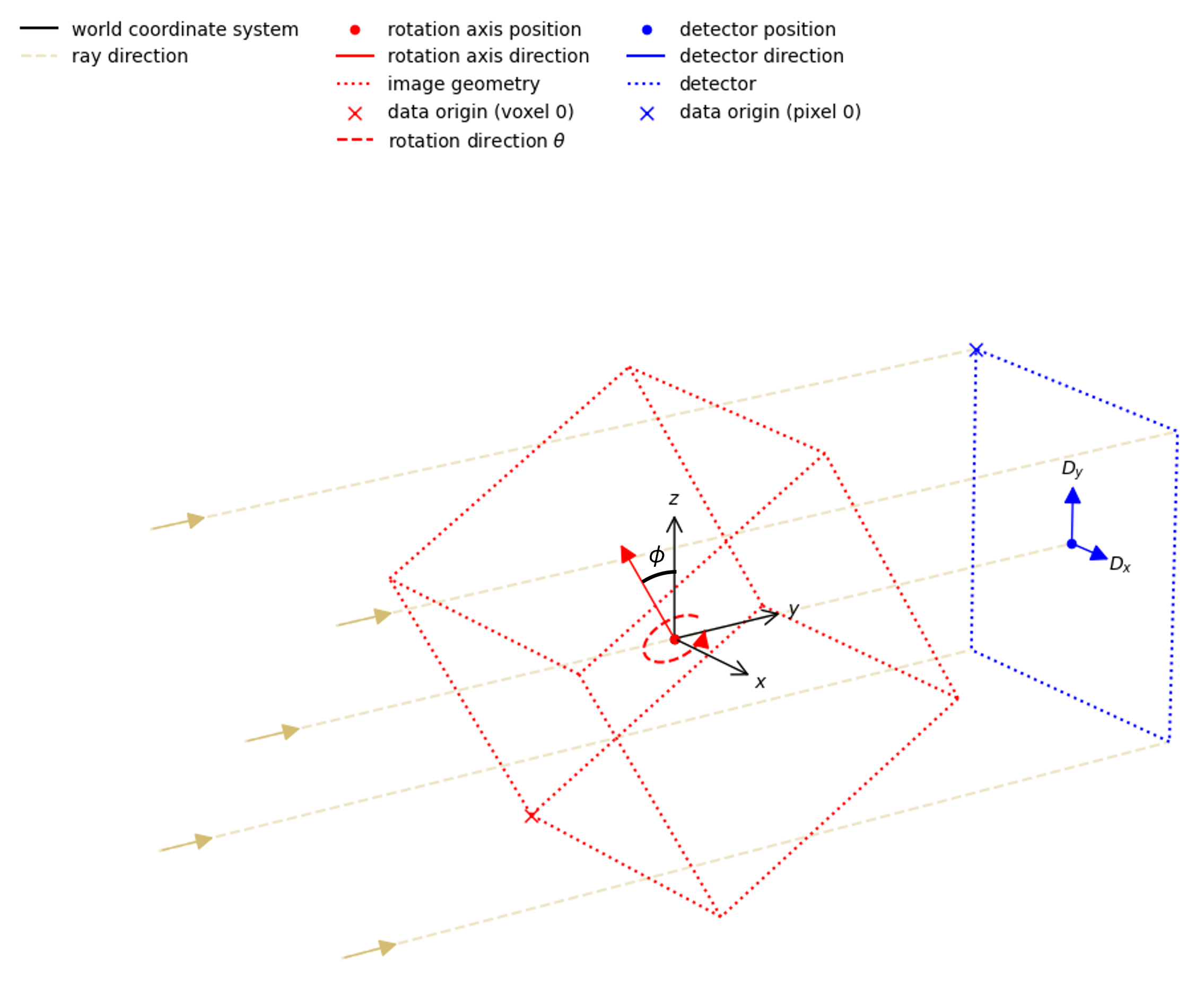
Laminography geometry from tilted rotation axis#
or equivalently by offsetting the source and detector:
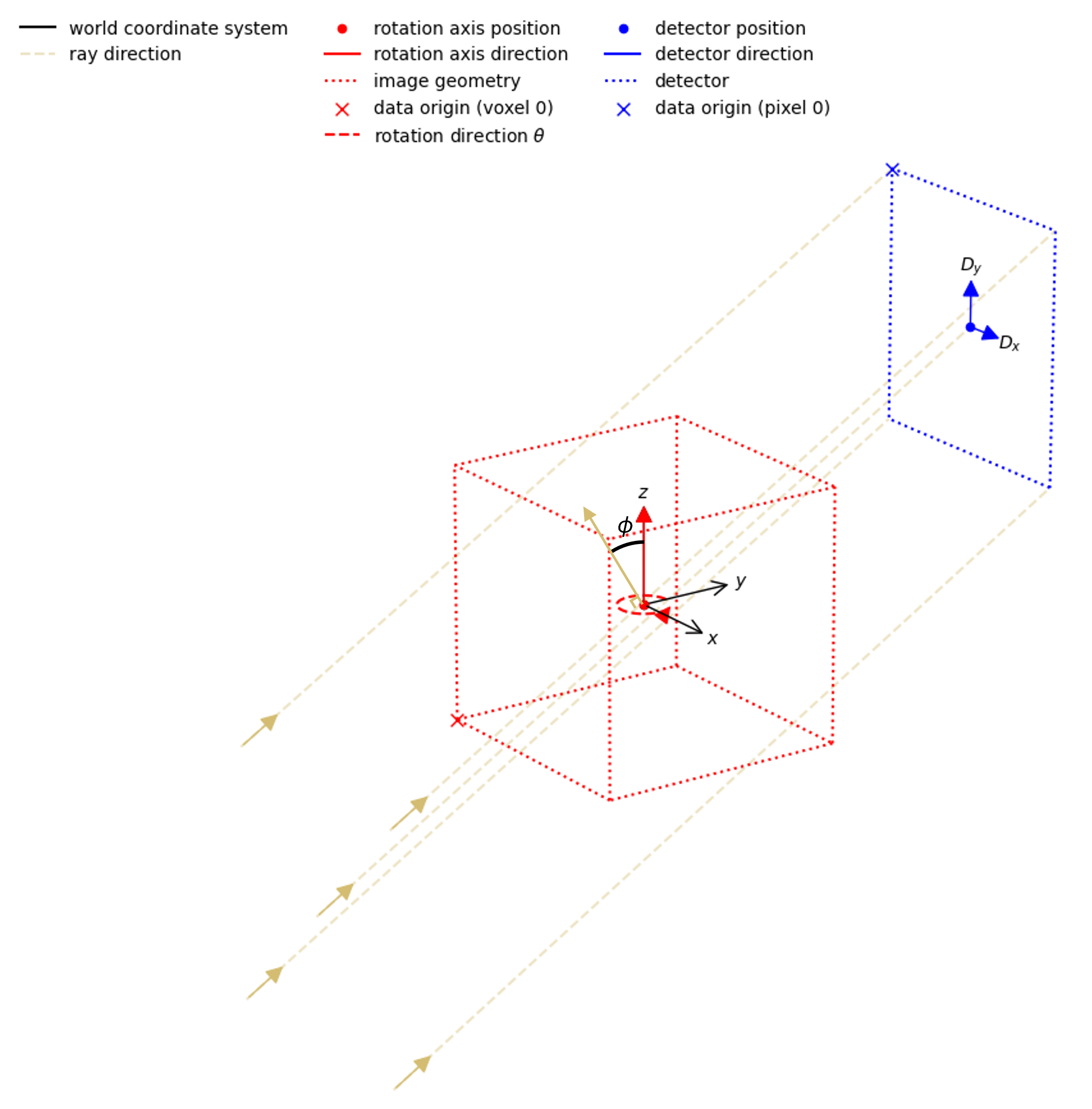
Laminography geometry from offset source and detector#
This processor fits the tilt angle \(\phi\) as well as the centre of rotation offset (defined above) for parallel beam laminography data.
- class cil.processors.LaminographyGeometryCorrector(parameter_bounds=[(-10, 10), (-20, 20)], parameter_tolerance=(0.01, 0.01), coarse_binning=None, final_binning=None, angle_subsampling=None, image_geometry=None, backend='astra')[source]#
LaminographyGeometryCorrector processor to fit the geometry of a parallel beam laminography dataset to find tilt and center-of-rotation.
- Parameters:
parameter_bounds (list of tuple of float, optional) – Bounds for the parameters [(tilt_min_deg, tilt_max_deg), (CoR_min_pix, CoR_max_pix)]. Defaults to [(-10, 10), (-20, 20)].
parameter_tolerance (tuple of float, optional) – Convergence tolerance for optimisation of parameters, (tilt_tol_deg, CoR_tol_pix). Defaults to (0.01, 0.01).
coarse_binning (int, optional) – Initial binning factor applied to the input dataset for coarse optimisation. If None, a value based on dataset size is used.
final_binning (int, optional) – Final binning factor applied for fine optimisation. If None, no binning is applied in the fine optimisation step.
angle_subsampling (float, optional) – Subsampling factor for the angle dimension during optimisation. If None, automatically determined based on input dataset.
image_geometry (ImageGeometry, optional) – Pass a reduced volume ImageGeometry to be used for fitting. If None, the full dataset is used.
backend ({'astra'}, optional) – The backend to use for the reconstruction. Currently only ‘astra’ is supported.
Example
>>> processor = LaminographyGeometryCorrector(parameter_bounds=(tilt_bounds, CoR_bounds),
    parameter_tolerance=(tilt_tol, CoR_tol))
>>> processor.set_input(data)
>>> data_corrected = processor.get_output()
- plot_evaluations()[source]#
Plot results from the minimisation. Plots the loss function value as a function of tilt and centre of rotation offset position.
- get_output(out=None)#
Runs the configured processor and returns the processed data
- Parameters:
out (DataContainer, optional) – Fills the referenced DataContainer with the processed data
- Returns:
The processed data
- Return type:
- set_input(dataset)#
Set the input data to the processor
- Parameters:
input (DataContainer) – The input DataContainer