[1]:
# -*- coding: utf-8 -*-
#  Copyright 2021 - 2022 United Kingdom Research and Innovation
#  Copyright 2021 - 2022 The University of Manchester
#
#  Licensed under the Apache License, Version 2.0 (the "License");
#  you may not use this file except in compliance with the License.
#  You may obtain a copy of the License at
#
#      http://www.apache.org/licenses/LICENSE-2.0
#
#  Unless required by applicable law or agreed to in writing, software
#  distributed under the License is distributed on an "AS IS" BASIS,
#  WITHOUT WARRANTIES OR CONDITIONS OF ANY KIND, either express or implied.
#  See the License for the specific language governing permissions and
#  limitations under the License.
#
#   Authored by:    Gemma Fardell (UKRI-STFC)
#                   Edoardo Pasca (UKRI-STFC)
#                   Laura Murgatroyd (UKRI-STFC)
A detailed look at CIL geometry#
CIL holds your CT data in specialised data-containers, AcquisitionData and ImageData.
Each of these has an associated geometry which contains the meta-data describing your set-up.
AcquisitionGeometrydescribes the acquisition data and parametersImageGeometrydescribes the image data (i.e., the reconstruction volume)
The data-readers provided by CIL (Nikon, Zeiss and diamond nexus readers) will read in your data and return you a fully configured acquisition data with the acquisition geometry already configured, however if you read in a stack of tiffs or want to tweak the parameters this is simple to create by hand.
The structure of an AcquisitionGeometry#
An instance of an AcquisitionGeometry, ag, holds the configuration of the system, in config which is subdivided in to:
ag.config.system- The position and orientations of thesource/ray,rotation_axisanddetectorag.config.panel- The number of pixels, the size of pixels, and the position of pixel 0ag.config.angles- The number of angles, the unit of the angles (default is degrees)ag.config.channels- The number of channels
Create a simple AcquisitionGeometry#
You can use the AcquisitionGeometry methods to describe circular trajectory parallel-beam or cone-beam 2D or 3D data.
ag = AcquisitionGeometry.create_Parallel2D()ag = AcquisitionGeometry.create_Parallel3D()ag = AcquisitionGeometry.create_Cone2D(source_position, detector_position)ag = AcquisitionGeometry.create_Cone3D(source_position, detector_position)
This notebook will step though each in turn and show you how to describe both simple and complex geometries with offsets and rotations.
No matter which type of geometry you create you will also need to describe the panel and projection angles.
ag.set_panel(num_pixels, pixel_size)ag.set_angles(angles, angle_unit)
For multi-channel data you need to add the number of channels.
ag.set_channels(num_channels)
And you will also need to describe the order your data is stored in using the relavent labels from the CIL default labels: channel, angle, vertical and horizontal
ag.set_labels(['angle','vertical','horizontal'])
A Note on CIL AcquisitionGeometry:#
The geometry is described by a right-handed cooridinate system
Positive angles describe the object rotating anti-clockwise when viewed from above
Parallel geometry#
Parallel beams of X-rays are emitted onto 1D (single pixel row) or 2D detector array. This geometry is common for synchrotron sources.
We describe the system, and then set the panel and angle data. Note that for 3D geometry we need to describe a 2D panel where num_pixels=[X,Y]
parallel_2D_geometry = AcquisitionGeometry.create_Parallel2D()\

                                          .set_panel(num_pixels=10)\

                                          .set_angles(angles=range(0,180))


parallel_3D_geometry = AcquisitionGeometry.create_Parallel3D()\

                                          .set_panel(num_pixels=[10,10])\

                                          .set_angles(angles=range(0,180))
Both 2D and 3D parallel-beam geometries are displayed below. Note that the detector position has been set, this is not necessary to describe and reconstruct the data, but it makes the displayed images clearer.
show_geometry() can be used to display the configured geometry and will be used here extensively. You can also print the geometry to obtain a detailed description. If show_geometry is not passed an ImageGeometry it will show the default geometry associated with the AcquisitionGeometry
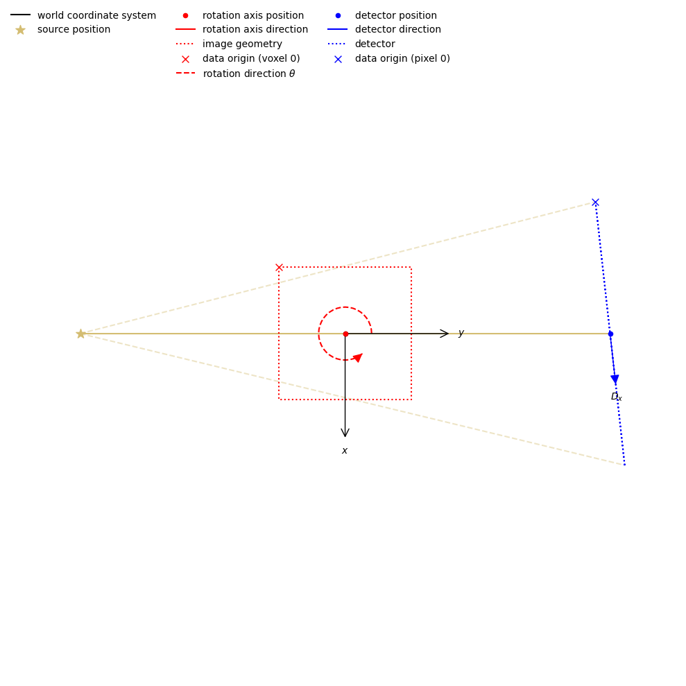
An example creating a 2D parallel-beam geometry:
[2]:
from cil.framework import AcquisitionGeometry
from cil.utilities.display import show_geometry

ag = AcquisitionGeometry.create_Parallel2D(detector_position=[0,10])\
    .set_panel(num_pixels=10)\
    .set_angles(angles=range(0,180))

show_geometry(ag)

print(ag)
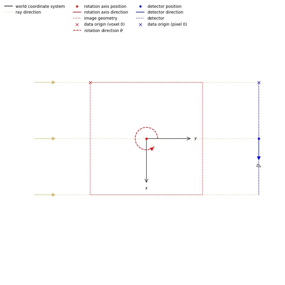
2D Parallel-beam tomography
System configuration:
        Ray direction: [0., 1.]
        Rotation axis position: [0., 0.]
        Detector position: [ 0., 10.]
        Detector direction x: [1., 0.]
Panel configuration:
        Number of pixels: [10  1]
        Pixel size: [1. 1.]
        Pixel origin: bottom-left
Channel configuration:
        Number of channels: 1
Acquisition description:
        Number of positions: 180
        Angles 0-9 in degrees: [0., 1., 2., 3., 4., 5., 6., 7., 8., 9.]
        Angles 170-179 in degrees: [170., 171., 172., 173., 174., 175., 176., 177., 178., 179.]
        Full angular array can be accessed with acquisition_data.geometry.angles
Distances in units: units distance
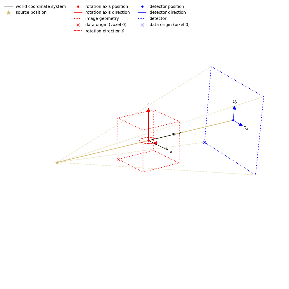
An example creating a 3D parallel-beam geometry:
[3]:
ag = AcquisitionGeometry.create_Parallel3D(detector_position=[0,10,0])\
    .set_panel(num_pixels=[10,10])\
    .set_angles(angles=range(0,180))

show_geometry(ag)
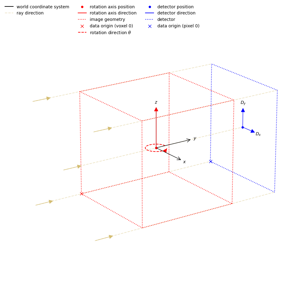
[3]:
<cil.utilities.display.show_geometry at 0x7f0394359160>
Fan-beam geometry#
A single point-like X-ray source emits a cone-beam onto a single row of detector pixels. The beam is typically collimated to imaging field of view. Collimation greatly reduce amount of scatter radiation reaching the detector. Fan-beam geometry is used when scattering has significant influence on image quality or single-slice reconstruction is sufficient.
We describe the system, and then set the panel and angle data.
For fan-beam data the source and detector positions are required. As default we place them along the Y-axis where the rotation-axis is on the origin. They are specified as [x,y] coordinates.
cone_2D_geometry = AcquisitionGeometry.create_Cone2D(source_position=[0,-10],detector_position=[0,10])\

                                      .set_panel(num_pixels=10)\

                                      .set_angles(angles=range(0,180))
[4]:
ag = AcquisitionGeometry.create_Cone2D(source_position=[0,-10],detector_position=[0,10])\
    .set_panel(num_pixels=10)\
    .set_angles(angles=range(0,180))

show_geometry(ag)
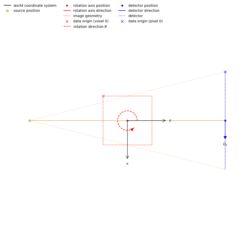
[4]:
<cil.utilities.display.show_geometry at 0x7f039416ed20>
Cone-beam geometry#
A single point-like X-ray source emits a cone-beam onto 2D detector array. Cone-beam geometry is mainly used in lab-based CT instruments.
We describe the system, and then set the panel and angle data.
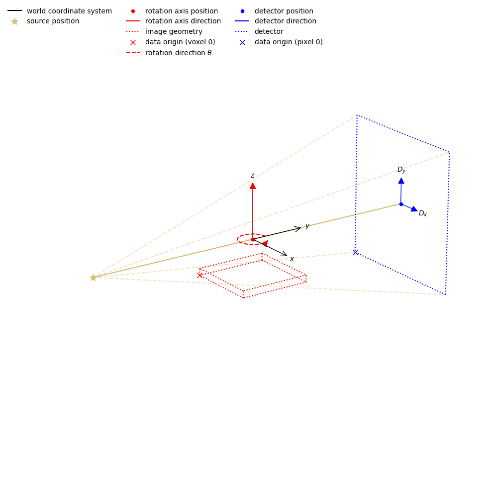
For cone-beam data the source and detector positions are required. As default we place them along the Y-axis where the rotation-axis is on the origin and aligned in the Z-direction. They are specified as [X,Y,Z] coordinates.
cone_3D_geometry = AcquisitionGeometry.create_Cone3D(source_position=[0,-10,0], detector_position=[0,10,0])\

                                      .set_panel(num_pixels=[10,10])\

                                      .set_angles(angles=range(0,180))
[5]:
ag = AcquisitionGeometry.create_Cone3D(source_position=[0,-10,0],detector_position=[0,10,0])\
    .set_panel(num_pixels=[10,10])\
    .set_angles(angles=range(0,180))

show_geometry(ag)
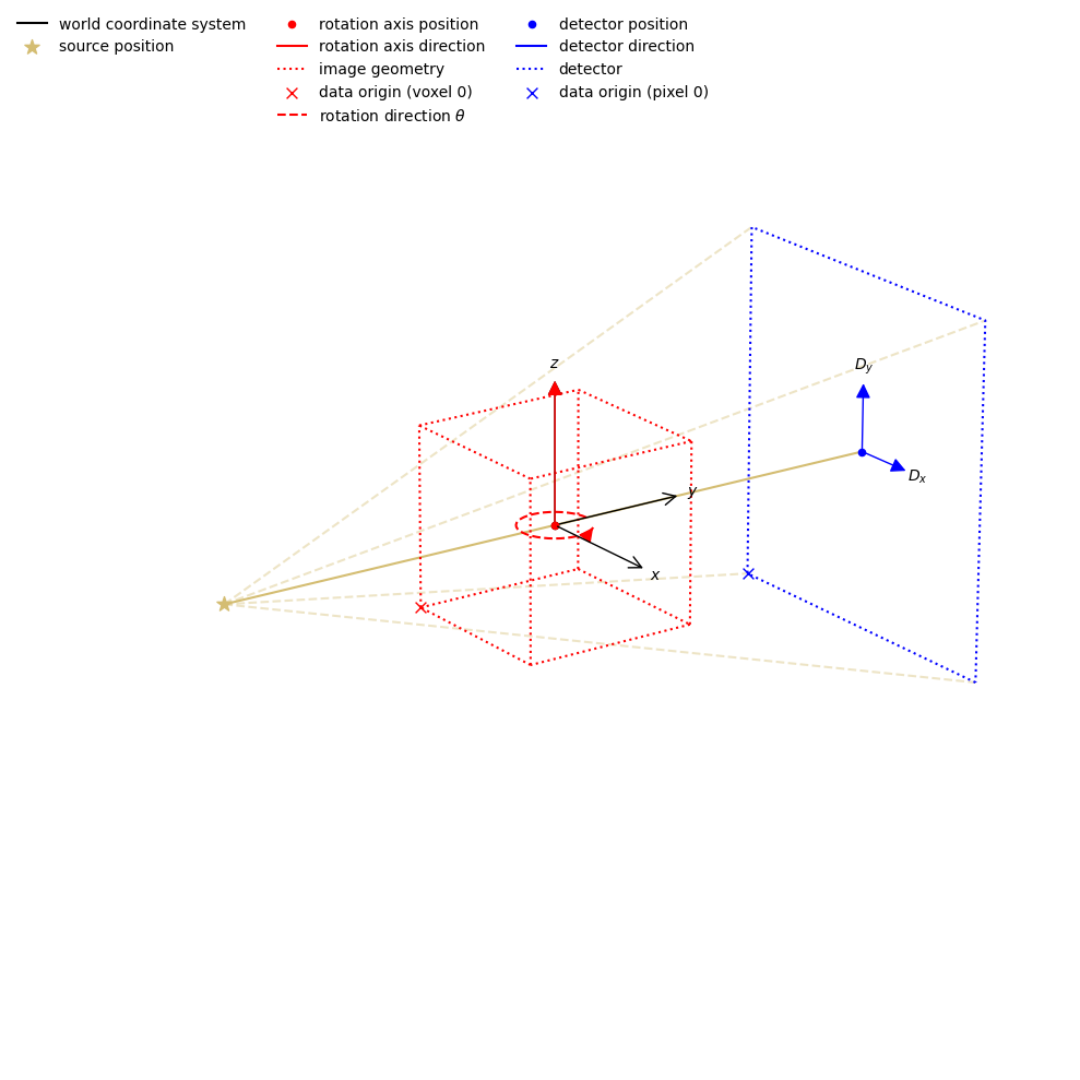
[5]:
<cil.utilities.display.show_geometry at 0x7f036bb5d8e0>
Create an offset AcquisitionGeometry#
It is unusual to have a perfectly aligned CT system. One of the most common offsets is the rotation-axis. If this offset is described by the AcquisitionGeometry then it will be accounted for in the reconstruction. This saves having to pad your data to account for this.
To specify the offset, you could either add an x-component to the source_position and detector_position or you can offset the rotation axis from the origin using rotation_axis_position.
As with the source_position and detector_position this is the rotation_axis_position is specified in 2D with a 2D vector [X,Y] or 3D with a 3D vector [X,Y,Z]
Below we offset the rotation axis by -0.5 in X by setting rotation_axis_position=[-0.5,0]. You can see the rotation axis position is no longer a point on the source-to-detector vector.
[6]:
ag = AcquisitionGeometry.create_Cone2D(source_position=[0,-10],detector_position=[0,10],
                                       rotation_axis_position=[-0.5,0])\
    .set_panel(num_pixels=10)\
    .set_angles(angles=range(0,180))

show_geometry(ag)

[6]:
<cil.utilities.display.show_geometry at 0x7f039428fc80>
Create a more complex AcquisitionGeometry#
We can also set up rotations in the system. These are configured with vectors describing the direction.
For example a detector yaw can be described by using detector_direction_x=[X,Y].
[7]:
ag = AcquisitionGeometry.create_Cone2D(source_position=[0,-10],detector_position=[0,10],
                                       detector_direction_x=[0.9,0.1]
                                       )\
     .set_panel(num_pixels=10)\
     .set_angles(angles=range(0,180))

show_geometry(ag)
[7]:
<cil.utilities.display.show_geometry at 0x7f039432dfd0>
You can set rotation_axis_direction, detector_direction_x and detector_direction_y by specifying a 3D directional vector [X,Y,Z].
For 3D datasets detector roll is commonly corrected with a dual-slice centre of rotation algorithm. You can specify detector_direction_x and detector_direction_y - ensuring they are ortogonal vectors.
[8]:
ag = AcquisitionGeometry.create_Cone3D(source_position=[0,-500,0],detector_position=[0,500,0],
                                       detector_direction_x=[0.9,0.0,-0.1],detector_direction_y=[0.1,0,0.9]
                                      )\
    .set_panel(num_pixels=[2048,2048], pixel_size = 0.2)\
    .set_angles(angles=range(0,180))

show_geometry(ag)
[8]:
<cil.utilities.display.show_geometry at 0x7f036b707da0>
In 3D datasets we can tilt the rotation axis to describe laminograpy geometry by changing rotation_axis_direction
[9]:
ag = AcquisitionGeometry.create_Cone3D(source_position=[0,-500,0],detector_position=[0,500,0],rotation_axis_direction=[0,-1,1])\
    .set_panel(num_pixels=[2048,2048], pixel_size = 0.2)\
    .set_angles(angles=range(0,180))

show_geometry(ag)
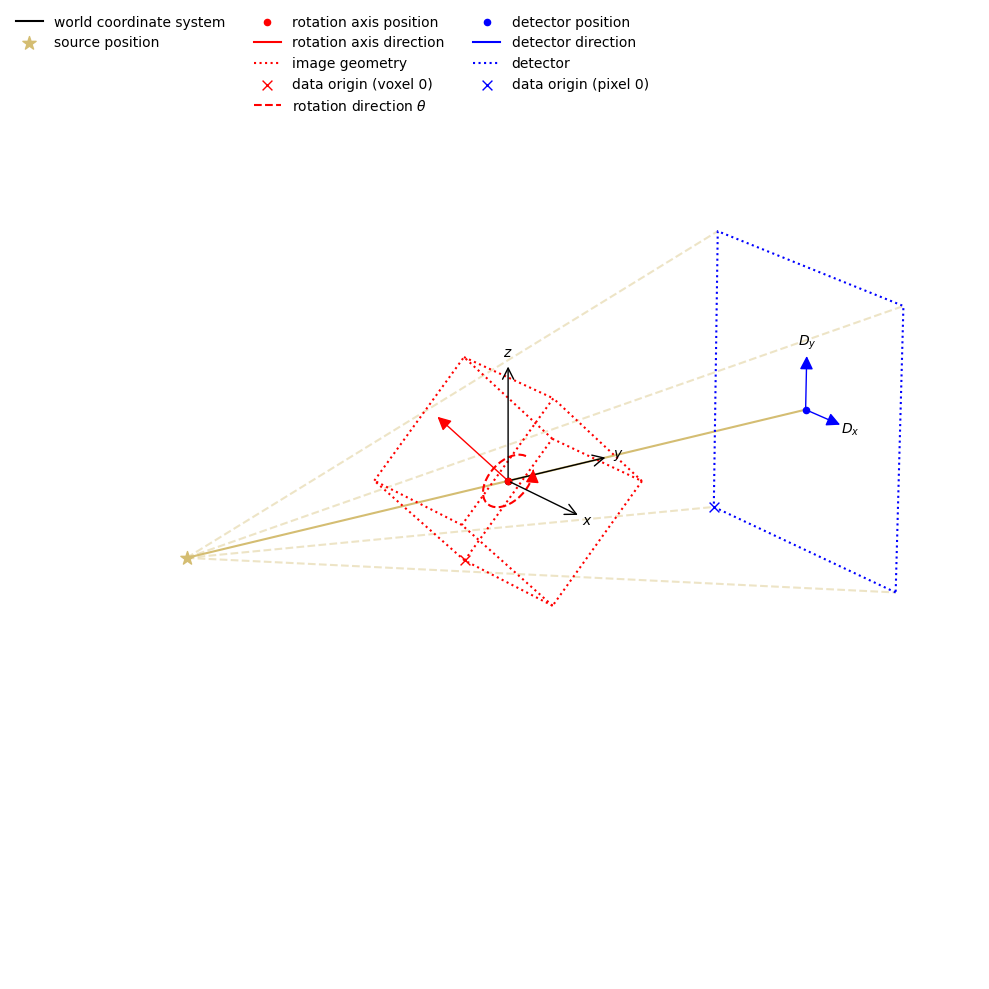
[9]:
<cil.utilities.display.show_geometry at 0x7f03942bd8e0>
The structure of an ImageGeometry#
ImageGeometry holds the description of the reconstruction volume. It holds:
The number of voxels in X, Y, Z:
voxel_num_x,voxel_num_y,voxel_num_zThe size of voxels in X, Y, Z:
voxel_size_x,voxel_size_y,voxel_size_zThe offset of the volume from the rotation axis in voxels:
center_x,center_y,center_zThe number of channels for multi-channel data
You will also need to describe the order your data is stored in using the relevent labels from the CIL. The default labels are: channel, vertical, horizontal_y and horizontal_x
ig.set_labels(['vertical','horizontal_y','horizontal_x'])
Create a simple ImageGeometry#
To create a default ImageGeometry you can use: ig = ag.get_ImageGeometry()
This creates an ImageGeometry with:
voxel_num_x,voxel_num_yequal to the number of horizontal pixels of the panelvoxel_num_zequal to the number of vertical pixels of the panelvoxel_size_x,voxel_size_yis given by the horizontal pixel size divided by magnificationvoxel_size_zis given by the vertical pixel size divided by magnification
You can pass a resolution argument: ig = ag.get_ImageGeometry(resolution)
resolution=0.5double the size of your voxels, and half the number of voxels in each dimensionresolution=2half the size of your voxels, and double the number of voxels in each dimension
A Note on CIL ImageGeometry:#
At 0 degrees horizontal_y is aligned with the Y axis, and horizontal_x with the X axis.
[10]:
ag = AcquisitionGeometry.create_Cone3D(source_position=[0,-500,0],detector_position=[0,500,0])\
    .set_panel(num_pixels=[2048,2048], pixel_size = 0.2)\
    .set_angles(angles=range(0,180))

print("ImageGeometry - default")
ig = ag.get_ImageGeometry()
print(ig)

print("ImageGeometry - 0.5x resolution")
ig = ag.get_ImageGeometry(resolution=0.5)
print(ig)

print("ImageGeometry - 2x resolution")
ig = ag.get_ImageGeometry(resolution=2)
print(ig)
ImageGeometry - default
Number of channels: 1
channel_spacing: 1.0
voxel_num : x2048,y2048,z2048
voxel_size : x0.1,y0.1,z0.1
center : x0,y0,z0

ImageGeometry - 0.5x resolution
Number of channels: 1
channel_spacing: 1.0
voxel_num : x1024,y1024,z1024
voxel_size : x0.2,y0.2,z0.2
center : x0,y0,z0

ImageGeometry - 2x resolution
Number of channels: 1
channel_spacing: 1.0
voxel_num : x4096,y4096,z4096
voxel_size : x0.05,y0.05,z0.05
center : x0,y0,z0
Create a custom ImageGeometry#
You can create your own ImageGeometry with: ig = ImageGeometry(...)
Giving you full control over the parameters.
You can also change the members directly to reduce the reconstructed volume to exclude empty space.
Using the previous example, we now can specify a smaller region of interest to reconstruct. We can offset the region of interest from the origin by specifiying the physical distance.
[11]:
ag = AcquisitionGeometry.create_Cone3D(source_position=[0,-500,0],detector_position=[0,500,0])\
.set_panel(num_pixels=[2048,2048], pixel_size = 0.2)\
.set_angles(angles=range(0,180))
print("ImageGeometry - default")
ig = ag.get_ImageGeometry()
show_geometry(ag, ig)
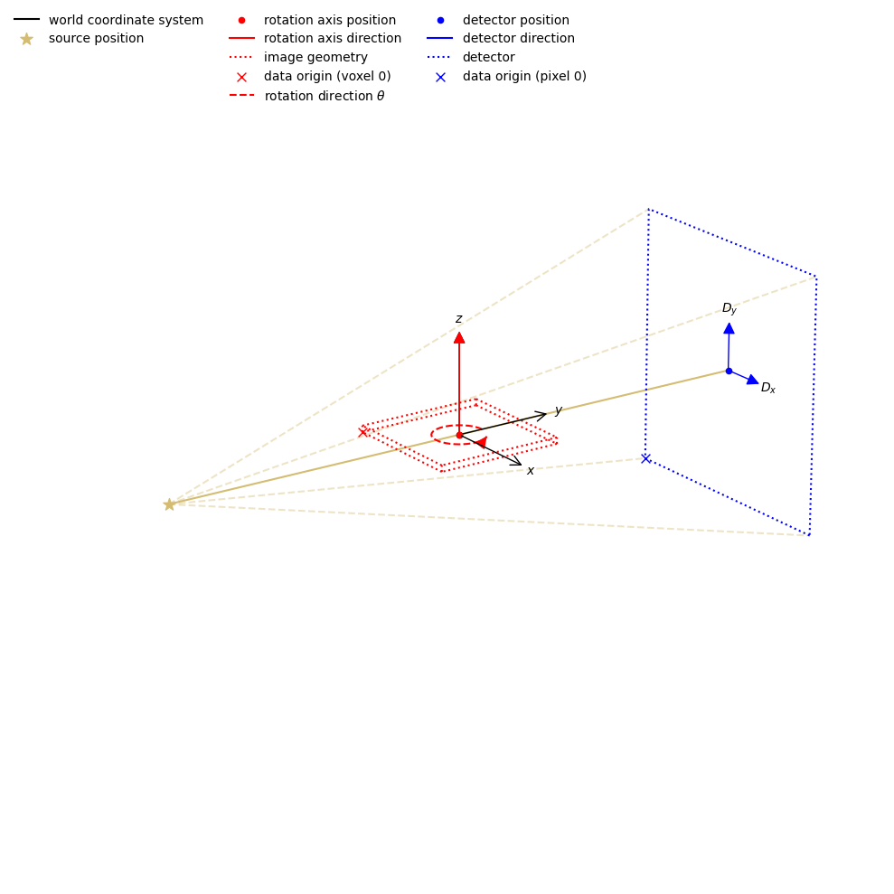
print("ImageGeometry - RoI")
ig = ag.get_ImageGeometry()
ig.voxel_num_z = 100
show_geometry(ag, ig)
print("ImageGeometry - Offset RoI")
ig = ag.get_ImageGeometry()
ig.voxel_num_z = 200
ig.center_z = -1024 * ig.voxel_size_z
show_geometry(ag, ig)
ImageGeometry - default

ImageGeometry - RoI
ImageGeometry - Offset RoI
[11]:
<cil.utilities.display.show_geometry at 0x7f039433b890>
We can also create an ImageGeometry directly.
Here we create our ig independently of an AcquisitionGeometry, by first importing ImageGeometry from cil.framework
[12]:
from cil.framework import ImageGeometry

ig = ImageGeometry(voxel_num_x=1000, voxel_num_y=1000, voxel_num_z=500, voxel_size_x=0.1, voxel_size_y=0.1, voxel_size_z=0.2 )